nolanessentials3e

11.2 One-Way Between-Groups ANOVA

279

The talking-while-driving study showed us that it’s dangerous when the person on the other end of the conversation doesn’t know when difficult driving conditions are developing. But we needed to analyze the data from four groups with an ANOVA to reach that conclusion. In this section, we use another four-group study to apply the principles of ANOVA to hypothesis testing with a between-groups research design.

Everything About ANOVA but the Calculations

To introduce the steps of hypothesis testing for a one-way between-groups ANOVA, we use an international study about whether the economic makeup of a society affects the degree to which people behave in a fair manner toward others (Henrich et al., 2010).

EXAMPLE 11.1

The researchers studied people in 15 societies from around the world. For teaching purposes, we’ll look at data from four types of societies—foraging, farming, natural resources, and industrial.

Foraging. Several societies, including ones in Bolivia and Papua New Guinea, were categorized as foraging societies. They acquired most of their food through hunting and gathering.
Farming. Some societies, including ones in Kenya and Tanzania, primarily practiced farming and tended to grow their own food.
Natural resources. Other societies, such as in Colombia, built their economies by extracting natural resources, such as trees and fish. Most food was purchased.
Industrial. In industrial societies, which include the major city of Accra in Ghana as well as rural Missouri in the United States, most food was purchased.

The researchers wondered which groups would behave more or less fairly toward others—the first and second groups, which grew their own food, or the third and fourth groups, which depended on others for food. The researchers measured fairness through several games. In the Dictator Game, for example, two players were given a sum of money equal to approximately the daily minimum wage for that society. The first player (the dictator) could keep all of the money or give any portion of it to the other person. The proportion of money given to the second player constituted the measure of fairness. For example, it would be considered fairer to give the second player 40% of the money than to give him or her only 10% of the money.

280

The Dictator Game Here a researcher introduces a fairness game to a woman fromPapua New Guinea, one of the foraging societies. Using games, researchers were able to compare fairness behaviors among different types of societies—those that depend on foraging, farming, natural resources, or industry. Because there are four groups and each participant is in only one group, the results can be analyzed with a one-way between-groups ANOVA.

This research design would be analyzed with a one-way between-groups ANOVA that uses the fairness measure, the proportion of money given to the second player, as the dependent variable. There is one independent variable (type of society) and it has four levels (foraging, farming, natural resources, and industrial). It is a between-groups design because each player lived in one and only one of those societies. It is an ANOVA because it analyzes variance by estimating the variability among the different types of societies and dividing it by the variability within the types of societies. The fairness scores below are from 13 fictional people, but the groups have almost the same mean fairness scores that the researchers observed in their actual (much larger) data set.

Foraging: 28, 36, 38, 31

Farming: 32, 33, 40

Natural resources: 47, 43, 52

Industrial: 40, 47, 45

Let’s begin by applying a familiar framework: the six steps of hypothesis testing. We will learn the calculations in the next section.

STEP 1: Identify the populations, distribution, and assumptions.

The first step of hypothesis testing is to identify the populations to be compared, the comparison distribution, the appropriate test, and the assumptions of the test. Let’s summarize the fairness study with respect to this first step of hypothesis testing.

Summary: The populations to be compared: Population 1: All people living in foraging societies. Population 2: All people living in farming societies. Population 3: All people living in societies that extract natural resources. Population 4: All people living in industrial societies.

The comparison distribution and hypothesis test: The comparison distribution will be an F distribution. The hypothesis test will be a one-way between-groups ANOVA.

281

Assumptions: (1) The data are not selected randomly, so we must generalize only with caution. (2) We do not know if the underlying population distributions are normal, but the sample data do not indicate severe skew. (3) We will test homoscedasticity when we calculate the test statistics by checking to see whether the largest variance is not more than twice the smallest. (Note: Don’t forget this step just because it comes later in the analysis.)

STEP 2: State the null and research hypotheses.

The second step is to state the null and research hypotheses. As usual, the null hypothesis posits no difference among the population means. The symbols are the same as before, but with more populations: H₀: μ₁ = μ₂ = μ₃ = μ₄. However, the research hypothesis is more complicated because we can reject the null hypothesis if only one group is different, on average, from the others. The research hypothesis that μ₁ ≠ μ₂ ≠ μ₃ ≠ μ₄ does not include all possible outcomes, such as the hypothesis that the mean fairness scores for groups 1 and 2 are greater than the mean fairness scores for groups 3 and 4. The research hypothesis is that at least one population mean is different from at least one other population mean, so H₁is that at least one µ is different from another µ.

Summary: Null hypothesis: People living in societies based on foraging, farming, the extraction of natural resources, and industry all exhibit, on average, the same fairness behaviors—H₀: μ₁ = μ₂ = μ₃ = μ₄. Research hypothesis: People living in societies based on foraging, farming, the extraction of natural resources, and industry do not all exhibit the same fairness behaviors, on average.

STEP 3: Determine the characteristics of the comparison distribution.

The third step is to explicitly state the relevant characteristics of the comparison distribution. This step is an easy one in ANOVA because most calculations are in step 5. Here we merely state that the comparison distribution is an F distribution and provide the appropriate degrees of freedom. As we discussed, the F statistic is a ratio of two independent estimates of the population variance, between-groups variance and within-groups variance (both of which we calculate in step 5). Each variance estimate has its own degrees of freedom. The sample between-groups variance estimates the population variance through the difference among the means of the samples—four, in this case. The degrees of freedom for the between-groups variance estimate is the number of samples minus 1:

MASTERING THE FORMULA

11-1: The formula for the between-groups degrees of freedom is: df_between = N_groups − 1. We subtract 1 from the number of groups in the study.

df_between = N_groups − 1 = 4 − 1 = 3

Because there are four groups (foraging, farming, the extraction of natural resources, and industry), the between-groups degrees of freedom is 3.

MASTERING THE FORMULA

11-2: The formula for the within-groups degrees of freedom for a one-way between-groups ANOVA conducted with four samples is: df_within = df₁ + df₂ + df₃ + df₄. We sum the degrees of freedom for each of the four groups. We calculate degrees of freedom for each group by subtracting 1 from the number of people in that sample. For example, for the first group, the formula is: df₁ = n₁ − 1.

The sample within-groups variance estimates the variance of the population by averaging the variances of the samples, without regard to differences among the sample means. We first must calculate the degrees of freedom for each sample. Because there are four participants in the first sample (farming), we would calculate:

df₁ = n₁ − 1 = 4 − 1 = 3

n represents the number of participants in the particular sample. We would then do this for the remaining samples. For this example, there are four samples, so the formula would be:

df_within = df₁ + df₂ + df₃ + df₄

282

For this example, the calculations would be:

df₁ = 4 − 1 = 3

df₂ = 3 − 1 = 2

df₃ = 3 − 1 = 2

df₄ = 3 − 1 = 2

df_within = 3 + 2 + 2 + 2 = 9

Summary: We would use the F distribution with 3 and 9 degrees of freedom.

STEP 4: Determine the critical value, or cutoff.

The fourth step is to determine a critical value, or cutoff, indicating how extreme the data must be to reject the null hypothesis. For ANOVA, we use an F statistic, for which the critical value on an F distribution will always be positive (because the F is based on estimates of variance and variances are always positive). We determine the critical value by examining the F table in Appendix B (excerpted in Table 11-3). 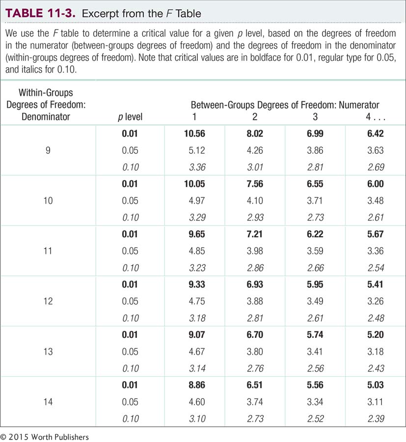The between-groups degrees of freedom are found in a row across the top of the table. Notice that, in the full table, this row only goes up to 6, as it is rare to have more than 7 conditions, or groups, in a study. The within-groups degrees of freedom are in a column along the left-hand side of the table. Because the number of participants in a study can range from a few to many, the column continues for several pages, with the same range of values of between-groups degrees of freedom on the top of each page.

283

Use the F table by first finding the appropriate within-groups degrees of freedom along the left-hand side of the page: 9. Then find the appropriate between-groups degrees of freedom along the top: 3. The place in the table where this row and this column intersect contains three numbers: p levels for 0.01, 0.05, and 0.10. Researchers usually use the middle one, 0.05, which for this study is 3.86 (Figure 11-2).

Figure 11.5: FIGURE 11-2
Determining Cutoffs for an F Distribution
We determine a single critical value on an F distribution. Because F is a squared version of a z (or t in some circumstances), we have only one cutoff for a two-tailed test.

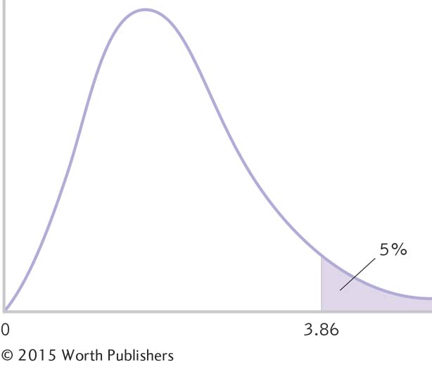
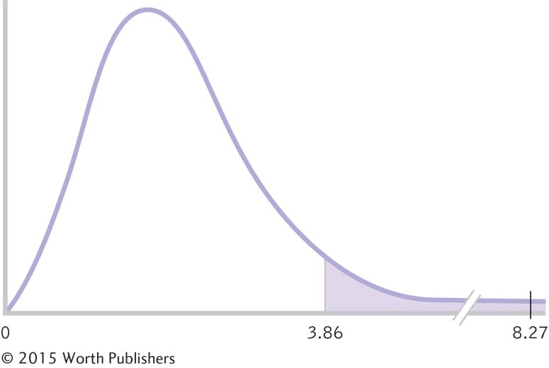
Summary: The cutoff, or critical value, for the F statistic for a p level of 0.05 is 3.86, as displayed in the curve in Figure 11-2.

STEP 5: Calculate the test statistic.

In the fifth step, we calculate the test statistic. We use the two estimates of the between-groups variance and the within-groups variance to calculate the F statistic. We compare the F statistic to the cutoff to determine whether to reject the null hypothesis. We will learn to do these calculations in the next section.

Summary: To be calculated in the next section.

STEP 6: Make a decision.

In the final step, we decide whether to reject or fail to reject the null hypothesis. If the F statistic is beyond the critical value, then we know that it is in the most extreme 5% of possible test statistics if the null hypothesis is true. We can then reject the null hypothesis and conclude, “It seems that people exhibit different fairness behaviors, on average, depending on the type of society in which they live.” ANOVA only tells us that at least one mean is significantly different from another; it does not tell us which societies are different.

MASTERING THE CONCEPT

11-2: When conducting an ANOVA, we use the same six steps of hypothesis testing that we’ve already learned. One of the differences from what we’ve learned is that we calculate an F statistic, the ratio of between-groups variance to within-groups variance.

If the test statistic is not beyond the critical value, then we must fail to reject the null hypothesis. The test statistic would not be very rare if the null hypothesis were true. In this circumstance, we report only that there is no evidence from the present study to support the research hypothesis.

Summary: Because the decision we will make must be evidence-based, we cannot make it until we complete step 5, in which we calculate the probabilities associated with that evidence. We will complete step 6 in the Making a Decision section.

The Logic and Calculations of the F Statistic

In this section, we first review the logic behind ANOVA’s use of between-groups variance and within-groups variance. Then we apply the same six steps of hypothesis testing we have used in previous statistical tests to make a data-driven decision about what story the data are trying to tell us. Our goal in performing the calculations of ANOVA is to understand the sources of all the variability in a study.

As we noted before, grown men, on average, are slightly taller than grown women, on average. We call that “between-groups variability.” We also noted that not all women are the same height and not all men are the same height. We call that “within-groups variability.” The F statistic is simply an estimate of between-groups variability (in the numerator) divided by an estimate of within-groups variability (in the denominator).

284

Gender Differences in Height Men, on average, are slightly taller than women (between-groups variance). However, neither men nor women are all the same height within their groups (within-groups variance). F is between-groups variability divided by within-groups variability.

Quantifying Overlap with ANOVA On average, men are taller than women; however, many women are taller than many men, so their distributions overlap. The amount of overlap is influenced by the distance between the means (between-groups variability) and the amount of spread (within-groups variability). In Figure 11-3a, there is a great deal of overlap; the means are close together and the distributions are spread out. Distributions with a lot of overlap suggest that any differences among them are probably due to chance.

Figure 11.6: FIGURE 11-3
The Logic of ANOVA
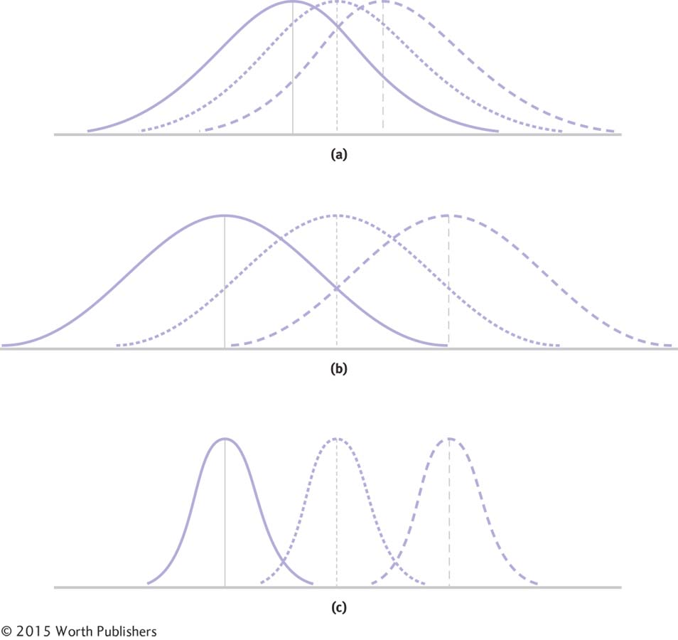
Compare the top (a) and middle (b) sets of sample distributions. As the variability between means increases, the F statistic becomes larger. Compare the middle (b) and bottom (c) sets of sample distributions. As the variability within the samples themselves decreases, the F statistic becomes larger because there is less overlap between the three curves. Both the increased spread among the sample means and the decreased spread within each sample contribute to this increase in the F statistic.

There is less overlap in the second set of distributions (see Figure 11-3b), but only because the means are farther apart; the within-groups variability remains the same. The F statistic is larger because the numerator is larger; the denominator has not changed. Distributions with little overlap are less likely to be drawn from the same population. It is less likely that any differences among them are due to chance.

There is even less overlap in the third set of distributions (see Figure 11-3c) because the numerator representing the between-groups variance is still large and the denominator representing the within-groups variance has gotten smaller. Both changes contributed to a larger F statistic. Distributions with very little overlap suggest that any differences are probably not due to chance. It would be difficult to convince someone that these three samples were drawn by chance from the very same population.

Two Ways to Estimate Population Variance Between-groups variability and within-groups variability estimate two different kinds of variance in the population. If those two estimates are the same, then the F statistic will be 1.0. For example, if the estimate of the between-groups variance is 32 and the estimate of the within-groups variance is also 32, then the F statistic is 32/32 = 1.0. This is a bit different from the z and t tests, in which a z or t of 0 would mean no difference at all. Here, an F of 1 means no difference at all. As the sample means get farther apart, the between-groups variance (the numerator) increases, which means that the F statistic also increases.

285

A source table presents the important calculations and final results of an ANOVA in a consistent and easy-to-read format.

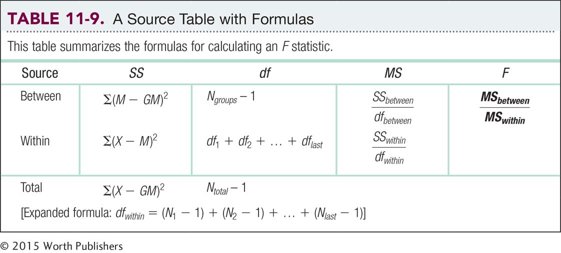
Calculating the F Statistic with the Source Table The goal of any statistical analysis is to understand the sources of variability in a study. We achieve that in ANOVA by calculating many squared deviations from the mean and three sums of squares. We organize the results into a source table that presents the important calculations and final results of an ANOVA in a consistent and easy-to-read format. A source table is shown in Table 11-4; the symbols in this table would be replaced by numbers in an actual source table. We’re going to explain the source table displayed in Table 11-4 starting with column 1; we will then work backward from column 5 to column 4 to column 3 and finally to column 2.

Column 1: “Source.” One possible source of population variance comes from the spread between means; a second source comes from the spread within each sample. In this chapter, the row labeled “Total” allows us to check the calculations of the sum of squares (SS) and degrees of freedom (df). Now let’s work backward through the source table to learn how it describes these two familiar sources of variability.

286

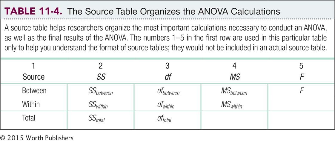
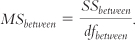
Column 5: “F.” We calculate F using simple division: between-groups variance divided by within-groups variance.

Column 4: “MS.” MS is the conventional symbol for variance in ANOVA. It stands for “mean square” because variance is the arithmetic mean of the squared deviations for between-groups variance (MS_between) and within-groups variance (MS_within). We divide MS_between by MS_within to calculate F.

MASTERING THE FORMULA

11-3: One formula for the total degrees of freedom for a one-way between-groups ANOVA is: df_total + df_between + df_within. We sum the between-groups degrees of freedom and the within-groups degrees of freedom. An alternate formula is: df_total = N_total − 1. We subtract 1 from the total number of people in the study—that is, from the number of people in all groups.

Column 3: “df.” We calculate the between-groups degrees of freedom (df_between) and the within-groups degrees of freedom (df_within), and then add the two together to calculate the total degrees of freedom:

df_total = df_between + df_within

In our version of the fairness study, df_total = 3 + 9 = 12. A second way to calculate df_total is:

df_total = N_total − 1

N_total refers to the total number of people in the entire study. In our abbreviated version of the fairness study, there were four groups, with 4, 3, 3, and 3 participants in the groups, and 4 + 3 + 3 + 3 = 13. We calculate total degrees of freedom for this study as df_total = 13 − 1 = 12. If we calculate degrees of freedom both ways and the answers don’t match up, then we know we have to go back and check the calculations.

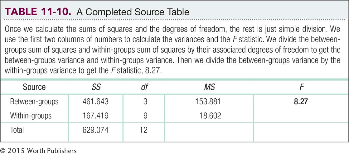
Column 2: “SS.” We calculate three sums of squares. One SS represents between-groups variability (SS_between), a second represents within-groups variability (SS_within), and a third represents total variability (SS_total). The first two sums of squares add up to the third; calculate all three to be sure they match.

The source table is a convenient summary because it describes everything we have learned about the sources of numerical variability. Once we calculate the sums of squares for between-groups variance and within-groups variance, there are just two steps.

Step 1: Divide each sum of squares by the appropriate degrees of freedom—the appropriate version of (N − 1). We divide the SS_between by the df_between and the SS_within by the df_within. We then have the two variance estimates (MS_between and MS_within).

Step 2: Calculate the ratio of MS_between and MS_within to get the F statistic. Once we have the sums of squared deviations, the rest of the calculation is simple division.

Sums of Squared Deviations Language Alert! The term “deviations” is another word used to describe variability. ANOVA analyzes three different types of statistical deviations: (1) deviations between groups, (2) deviations within groups, and (3) total deviations. We begin by calculating the sum of squares for each type of deviation, or source of variability: between, within, and total.

287

It is easiest to start with the total sum of squares, SS_total. Organize all the scores and place them in a single column with a horizontal line dividing each sample from the next. Use the data (from our version of the fairness study) in the column labeled “X” of Table 11-5 as a model; X stands for each of the 13 individual scores listed below. Each set of scores is next to its sample; the means are underneath the names of each respective sample. 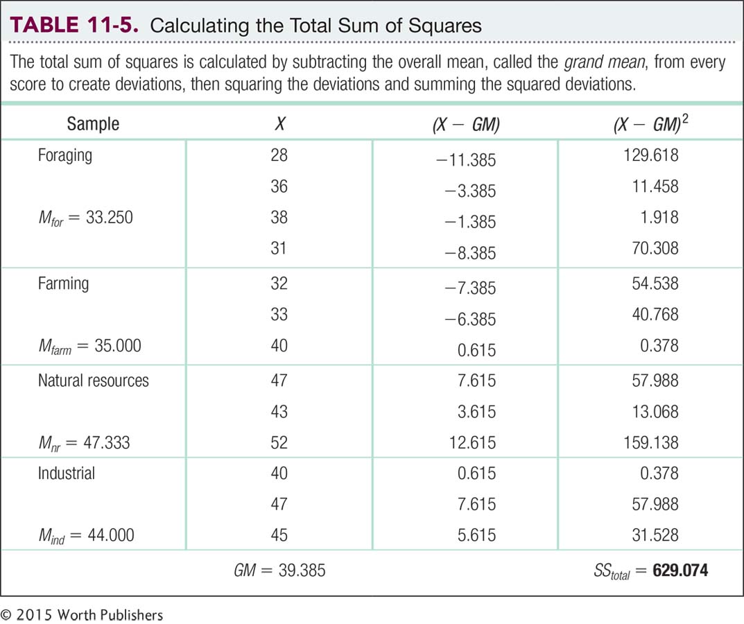(We have included subscripts on each mean in the first column—e.g., for for foraging, nr for natural resources—to indicate its sample.)

The grand mean is the mean of every score in a study, regardless of which sample the score came from.

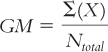
To calculate the total sum of squares, subtract the overall mean from each score, including everyone in the study, regardless of sample. The mean of all the scores is called the grand mean, and its symbol is GM. The grand mean is the mean of every score in a study, regardless of which sample the score came from:

MASTERING THE FORMULA

11-4: The grand mean is the mean score of all people in a study, regardless of which sample the score came from. The formula is:

We add up everyone’s score, then divide by the total number of people in the study.

The grand mean of these scores is 39.385. (As usual, we write each number to three decimal places until we get to the final answer, F. We report the final answer to two decimal places.)

The third column in Table 11-5 shows the deviation of each score from the grand mean. The fourth column shows the squares of these deviations. For example, for the first score, 28, we subtract the grand mean:

28 − 39.385 = −11.385

288

Then we square the deviation:

MASTERING THE FORMULA

11-5: The total sum of squares in an ANOVA is calculated using the following formula: SS_total = Σ(X − GM)². We subtract the grand mean from every score, then square these deviations. We then sum all the squared deviations.

(−11.385)² = 129.618

Below the fourth column, we have summed the squared deviations: 629.074. This is the total sum of squares, SS_total. The formula for the total sum of squares is:

SS_total = Σ(X − GM)²

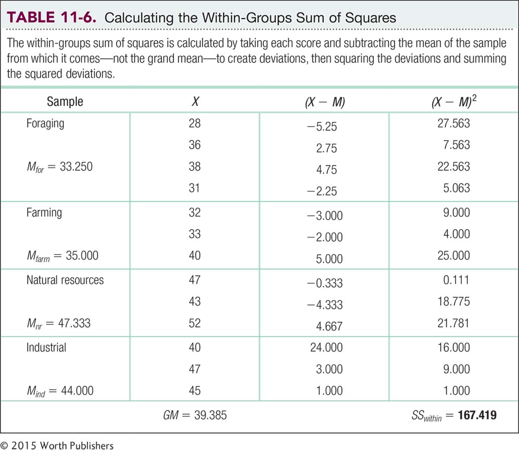
The model for calculating the within-groups sum of squares is shown in Table 11-6. This time the deviations are around the mean of each particular group (separated by horizontal lines) instead of around the grand mean. For the four scores in the first sample, we subtract their sample mean, 33.25. For example, the calculation for the first score is:

(28 − 33.25)² = 27.563

MASTERING THE FORMULA

11-6: The within-groups sum of squares in a one-way between-groups ANOVA is calculated using the following formula: SS_within = Σ(X − M)². From each score, we subtract its group mean. We then square these deviations. We sum all the squared deviations for everyone in all groups.

For the three scores in the second sample, we subtract their sample mean, 35.0. And so on for all four samples. (Note: Don’t forget to switch means when you get to each new sample!)

Once we have all the deviations, we square them and sum them to calculate the within-groups sum of squares, 167.419, the number below the fourth column. Because we subtract the sample mean, rather than the grand mean, from each score, the formula is:

SS_within = Σ(X − M)²

289

Notice how the weighting for sample size is built into the calculation: The first sample has four scores and contributes four squared deviations to the total. The other samples have only three scores, so they only contribute three squared deviations.

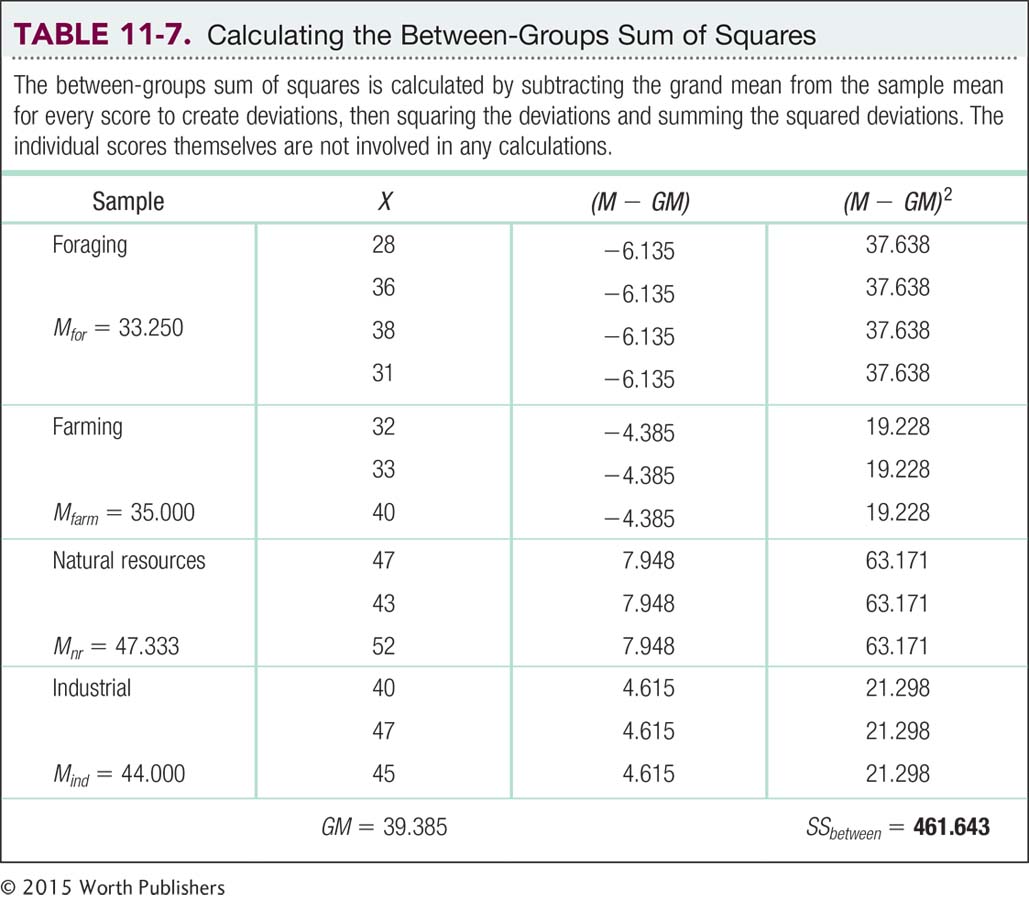
Finally, we calculate the between-groups sum of squares. Remember, the goal for this step is to estimate how much each group—not each individual participant—deviates from the overall grand mean, so we use means rather than individual scores in the calculations. For each of the 13 people in this study, we subtract the grand mean from the mean of the group to which that individual belongs.

For example, the first person has a score of 28 and belongs to the group labeled “foraging,” which has a mean score of 33.25. The grand mean is 39.385. We ignore this person’s individual score and subtract 39.385 (the grand mean) from 33.25 (the group mean) to get the deviation score, −6.135. The next person, also in the group labeled “foraging,” has a score of 36. The group mean of that sample is 33.25. Once again, we ignore that person’s individual score and subtract 39.385 (the grand mean) from 33.25 (the group mean) to get the deviation score, also −6.135.

In fact, we subtract 39.385 from 33.25 for all four scores, as you can see in Table 11-7. When we get to the horizontal line between samples, we look for the next sample mean. For all three scores in the next sample, we subtract the grand mean, 39.385, from the sample mean, 35.0, and so on.

MASTERING THE FORMULA

11-7: The between-groups sum of squares in an ANOVA is calculated using the following formula: SS_between = Σ(M − GM)². For each score, we subtract the grand mean from that score’s group mean, and square this deviation. Note that we do not use the scores in any of these calculations. We sum all the squared deviations.

Notice that individual scores are never involved in the calculations, just sample means and the grand mean. Also notice that the first group (foraging), with four participants, has more weight in the calculation than the other three groups, which each have only three participants. The third column of Table 11-7 includes the deviations and the fourth includes the squared deviations. The between-groups sum of squares, in bold under the fourth column, is 461.643. The formula for the between-groups sum of squares is:

SS_between = Σ (M − GM)²

290

Now is the moment of arithmetic truth. Were the calculations correct? To find out, we add the within-groups sum of squares (167.419) to the between-groups sum of squares (461.643) to see if they equal the total sum of squares (629.074). Here’s the formula:

SS_total = SS_within + SS_between = 629.062 = 167.419 + 461.643

Indeed, the total sum of squares, 629.074, is almost equal to the sum of the other two sums of squares, 167.419 and 461.643, which is 629.062. The slight difference is due to rounding decisions. So the calculations were correct.

MASTERING THE FORMULA

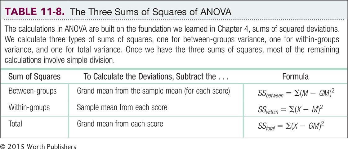
11-8: We can also calculate the total sum of squares for a one-way between-groups ANOVA by adding the within-groups sum of squares and the between-groups sum of squares: SS_total = SS_within + SS_between. This is a useful check on the calculations.

To recap (Table 11-8), for the total sum of squares, we subtract the grand mean from each individual score to get the deviations. For the within-groups sum of squares, we subtract the appropriate sample mean from every score to get the deviations. And for the between-groups sum of squares, we subtract the grand mean from the appropriate sample mean, once for each score, to get the deviations; for the between-groups sum of squares, the actual scores are never involved in any calculations.

MASTERING THE FORMULA

11-9: We calculate the mean squares from their associated sums of squares and degrees of freedom. For the between-groups mean square, we divide the between-groups sum of squares by the between-groups degrees of freedom:

For the within-groups mean square, we divide the within-groups sum of squares by the within-groups degrees of freedom:

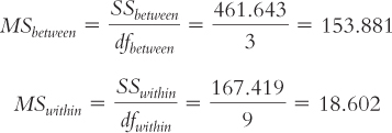
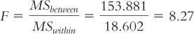
Now we insert these numbers into the source table to calculate the F statistic. See Table 11-9 for the source table that lists all the formulas and Table 11-10 for the completed source table. We divide the between-groups sum of squares and the within-groups sum of squares by their associated degrees of freedom to get the between-groups variance and the within-groups variance. The formulas are:

MASTERING THE FORMULA

11-10: The formula for the F statistic is:

We divide the between-groups mean square by the within-groups mean square.

We then divide the between-groups variance by the within-groups variance to calculate the F statistic. The formula, in bold in Table 11-9, is:

Making a Decision

Now we have to come back to the six steps of hypothesis testing for ANOVA to fill in the gaps in steps 1 and 6. We finished steps 2 through 5 in the previous section.

291

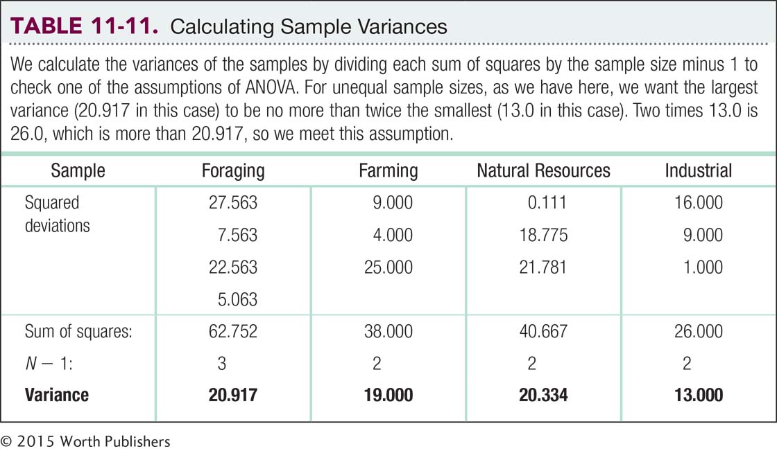
Step 1: ANOVA assumes that participants were selected from populations with equal variances. Statistical software, such as SPSS, tests this assumption while analyzing the overall data. For now, we can use the last column from the within-groups sum of squares calculations in Table 11-6. Variance is computed by dividing the sum of squares by the sample size minus 1. We can add the squared deviations for each sample, then divide by the sample size minus 1. Table 11-11 shows the calculations for variance within each of the four samples. Because the largest variance, 20.917, is not more than twice the smallest variance, 13.0, we have met the assumption of equal variances.

292

Step 6: Now that we have the test statistic, we compare it with 3.86, the critical F value that we identified in step 4. The F statistic we calculated was 8.27, and Figure 11-4 demonstrates that the F statistic is beyond the critical value: We can reject the null hypothesis. It appears that people living in some types of societies are fairer, on average, than are people living in other types of societies. And congratulations on making your way through your first ANOVA! Statistical software will do all of these calculations for you, but understanding how the computer produced those numbers adds to your overall understanding.

Figure 11.15: FIGURE 11-4
Making a Decision with an F Distribution
We compare the F statistic that we calculated for the samples to a single cutoff, or critical value, on the appropriate F distribution. We can reject the null hypothesis if the test statistic is beyond—more to the right than—the cutoff. Here, the F statistic of 8.27 is beyond the cutoff of 3.86, so we can reject the null hypothesis.

The ANOVA, however, only allows us to conclude that at least one mean is different from at least one other mean. The next section describes how to determine which groups are different.

Summary: We reject the null hypothesis. It appears that mean fairness levels differ based on the type of society in which a person lives. In a scientific journal, these statistics are presented in a similar way to the z and t statistics but with separate degrees of freedom in parentheses for between-groups and within-groups: F (3, 9) = 8.27, p < 0.05. (Note: Use the actual p value when analyzing ANOVA with statistical software.)

CHECK YOUR LEARNING

Reviewing the Concepts		One-way between-groups ANOVA uses the same six steps of hypothesis testing that we learned in Chapter 7, but with a few minor changes in steps 3 and 5. In step 3, we merely state the comparison distribution and provide two different types of degrees of freedom, df for the between-groups variance and df for the within-groups variance. In step 5, we complete the calculations, using a source table to organize the results. First, we estimate population variance by considering the differences among means (between-groups variance). Second, we estimate population variance by calculating a weighted average of the variances within each sample (within-groups variance). The calculation of variability requires several means, including sample means and the grand mean, which is the mean of all scores, regardless of which sample the scores came from. We divide between-groups variance by within-groups variance to calculate the F statistic. Before making a decision based on the F statistic, we check to see whether the assumption of equal sample variances is met. This assumption is met when the largest sample variance is not more than twice the amount of the smallest variance.
Clarifying the Concepts	11-5	If the F statistic is beyond the cutoff, what does that tell us? What doesn’t that tell us?
	11-6	What is the primary subtraction that enters into the calculation of SS_between?
Calculating the Statistics	11-7	Calculate each type of degrees of freedom for the following data, assuming a between-groups design: Group 1: 37, 30, 22, 29 Group 2: 49, 52, 41, 39 Group 3: 36, 49, 42 df_between = N_groups − 1 df_within = df₁ + df₂ + … + df_last df_total = df_between + df_within, or df_total = N_total − 1
	11-8	Using the data in Check Your Learning 11-7, compute the grand mean.
	11-9	Using the data in Check Your Learning 11-7, compute each type of sum of squares. Total sum of squares Within-groups sum of squares Between-groups sum of squares
	11-10	Using all of your calculations in Check Your Learning 11-7 to 11-9, perform the simple division to complete an entire between-groups ANOVA source table for these data.
Applying the Concepts	11-11	Let’s create a context for the data provided above. Hollon, Thase, and Markowitz (2002) reviewed the efficacy of different treatments for depression, including medications, electroconvulsive therapy, psychotherapy, and placebo treatments. These data re-create some of the basic findings the researchers present regarding psychotherapy. Each group is meant to represent people who received a different psychotherapy-based treatment, including psychodynamic therapy in group 1, interpersonal therapy in group 2, and cognitive-behavioral therapy in group 3. The scores presented here represent the extent to which someone responded to the treatment, with higher numbers indicating greater efficacy of treatment. Group 1 (psychodynamic therapy): 37, 30, 22, 29 Group 2 (interpersonal therapy): 49, 52, 41, 39 Group 3 (cognitive-behavioral therapy): 36, 49, 42 Write hypotheses, in words, for this research. Check the assumptions of ANOVA. Determine the critical value for F. Using your calculations from Check Your Learning 11-10, make a decision about the null hypothesis for these treatment options.

Solutions to these Check Your Learning questions can be found in Appendix D.