11.3 Beyond Hypothesis Testing for the One-Way Between-Groups ANOVA
Is driving while talking on a hands-
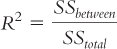
R2, the Effect Size for ANOVA
R2 is the proportion of variance in the dependent variable that is accounted for by the independent variable.
MASTERING THE CONCEPT
11-
MASTERING THE FORMULA
11-
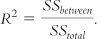
The calculation is a ratio, similar to the calculation for the F statistic. For R2, we divide the between-
In Chapter 8, we learned how to use Cohen’s d to calculate effect size. However, Cohen’s d only applies when subtracting one mean from another (as for a z test or a t test). With ANOVA, we calculate R2 (pronounced “r squared”), the proportion of variance in the dependent variable that is accounted for by the independent variable. We could also calculate a similar statistic called η2 (pronounced “eta squared”). We can interpret η2 exactly as we interpret R2.
Like the F statistic, R2 is a ratio. However, it calculates the proportion of variance accounted for by the independent variable out of all of the variance. Its numerator uses only the between-
EXAMPLE 11.2
Let’s apply this to the ANOVA we just conducted. We can use the statistics in the source table we created earlier to calculate R2:
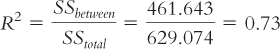
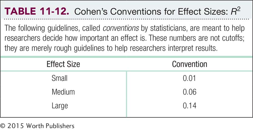
Table 11-12 displays Jacob Cohen’s conventions for R2 that, like Cohen’s d, indicate whether the effect size is small, medium, or large. This R2 of 0.73 is large. This is not surprising; if we can reject the null hypothesis when the sample size is small, then the effect size must be large. We can also turn the proportion into the more familiar language of percentages by multiplying by 100.
We can then say that a specific percentage of the variance in the dependent variable is accounted for by the independent variable. In this case, we could say that 73% of the variability in sharing is due to the type of society. (Note that our overall results match those of the original study; however, the actual effect size was lower than this.)
Post Hoc Tests
A post hoc test is a statistical procedure frequently carried out after the null hypothesis has been rejected in an analysis of variance; it allows us to make multiple comparisons among several means; often referred to as a follow-
up test .
The statistically significant F statistic means that some difference exists somewhere in the study. The R2 tells us that the difference is large, but we still don’t know which pairs of means are responsible for these effects. Here’s an easy way to figure it out: Graph the data. The picture will suggest which means are different, but those differences still need to be confirmed with a post hoc test. A post hoc test is a statistical procedure frequently carried out after the null hypothesis has been rejected in an analysis of variance; it allows us to make multiple comparisons among several means. The name of the test, post hoc, means “after this” in Latin; these tests are often referred to as follow-
MASTERING THE CONCEPT
11-
For example, the fairness study produced the following mean scores: foraging, 33.25; farming, 35.0; industrial, 44.0; and natural resources, 47.333. The ANOVA told us to reject the null hypothesis, so something is going on in this data set. The Pareto chart (organized by highest to lowest) and a post hoc test will tell us “where the action is” in this statistically significant ANOVA.
The graph in Figure 11-5 helps us think through the possibilities. For example, people in industrial societies and in societies that extract natural resources might exhibit higher levels of fairness, on average, than people in foraging or farming societies (groups 1 and 2 versus groups 3 and 4). Or people in societies that extract natural resources might be higher, on average, only compared with those in foraging societies (group 1 versus group 4). Maybe all four groups are different from one another, on average. There are so many possibilities that we need a post hoc test to reach a statistically valid conclusion. There are many post hoc tests and most are named for their founders, almost exclusively people with fabulous names—
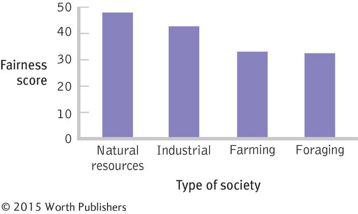
Which Types of Societies Are Different in Terms of Fairness?
This graph depicts the mean fairness scores of people living in each of four different types of societies. When we conduct an ANOVA and reject the null hypothesis, we only know that there is a difference somewhere; we do not know where the difference lies. We can see several possible combinations of differences by examining the means on this graph. A post hoc test will let us know which specific pairs of means are different from one another.
Tukey HSD
The Tukey HSD test is a widely used post hoc test that determines the differences between means in terms of standard error; the HSD is compared to a critical value; sometimes called the q test.
The Tukey HSD test is a widely used post hoc test that determines the differences between means in terms of standard error; the HSD is compared to a critical value. The Tukey HSD test (also called the q test) stands for “honestly significant difference” because it allows us to make multiple comparisons to identify differences that are “honestly” there.
MASTERING THE FORMULA
11-
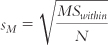 . We divide the MSwithin by the sample size and take the square root. We can then calculate the HSD for each pair of means:
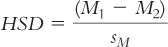
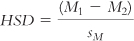 . For each pair of means, we subtract one from the other and divide by the standard error we calculated earlier.
In the Tukey HSD test, we (1) calculate differences between each pair of means, (2) divide each difference by the standard error, and (3) compare the HSD for each pair of means to a critical value (a q value, found in Appendix B) to determine whether the means are different enough to reject the null hypothesis. The formula for the Tukey HSD test is a variant of the z test and t tests for any two sample means:
The formula for the standard error is:
N in this case is the sample size within each group, with the assumption that all samples have the same number of participants.
MASTERING THE FORMULA
11-
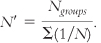
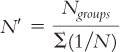
To do that, we divide the number of groups in the study by the sum of 1 divided by the sample size for every group.
When samples are different sizes, as in our example of societies, we have to calculate a weighted sample size, also known as a harmonic mean, N′ (pronounced “N prime”) before we can calculate standard error:
EXAMPLE 11.3
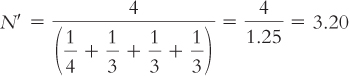
We calculate N′ by dividing the number of groups (the numerator) by the sum of 1 divided by the sample size for every group (the denominator). For the example in which there were four participants in foraging societies and three in each of the other three types of societies, the formula is:
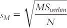
When sample sizes are not equal, we use a formula for sM based on N′ instead of N:
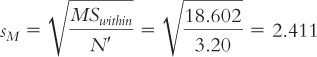
MASTERING THE FORMULA
11-
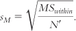
To do that, we divide MSwithin by N′ and take the square root.
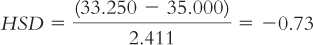
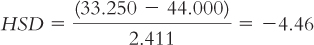
Now we use simple subtraction to calculate HSD for each pair of means. Which comes first doesn’t matter; for example, we could subtract the mean for foraging societies from the mean for farming societies, or vice versa—
Foraging (33.250) versus farming (35.000):
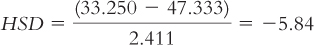
Foraging (33.250) versus natural resources (47.333):
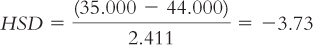
Foraging (33.250) versus industrial (44.000):
Farming (35.000) versus natural resources (47.333):
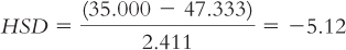
Farming (35.000) versus industrial (44.000):
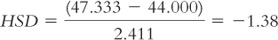
Natural resources (47.333) versus industrial (44.000):
Now all we need is a critical value from the q table in Appendix B (excerpted in Table 11-13) to which we can compare the HSDs. The numbers of means being compared (levels of the independent variable) are in a row along the top of the q table, and the within-
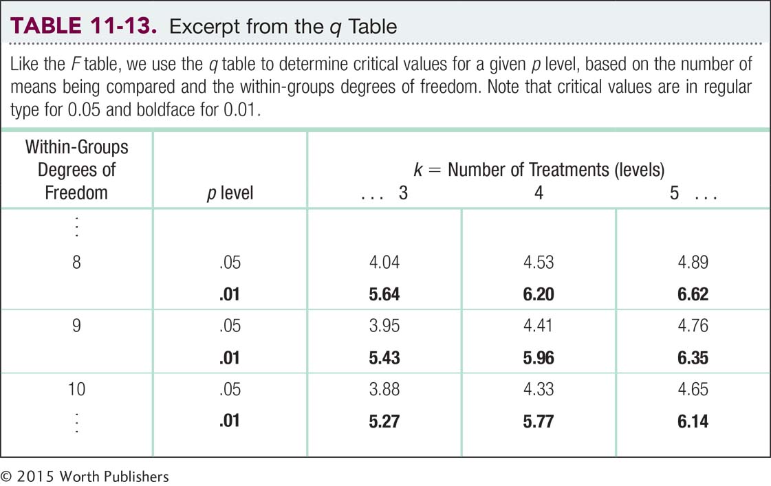
The q table indicates three statistically significant differences whose HSDs are beyond the critical value of −4.41: −5.84, −4.46, and −5.12. It appears that people in foraging societies are less fair, on average, than people in societies that depend on natural resources and people in industrial societies. In addition, people in farming societies are less fair, on average, than are people in societies that depend on natural resources. We have not rejected the null hypothesis for any other pairs, so we can only conclude that there is not enough evidence to determine whether their means are different.
What might explain these differences? The researchers observed that people who purchase food routinely interact with other people in an economic market. They concluded that higher levels of market integration are associated with higher levels of fairness (Henrich et al., 2010). Social norms of fairness may develop in market societies that require cooperative interactions between people who do not know each other.
How much faith can we have in these findings? Cautious confidence and replication are recommended; researchers could not randomly assign people to live in particular societies, so some third variable may explain the relation between market integration and fairness.
CHECK YOUR LEARNING
| Reviewing the Concepts |
|
|
| Clarifying the Concepts | 11- |
When do we conduct a post hoc test, such as a Tukey HSD test, and what does it tell us? |
| 11- |
How is R2 interpreted? | |
| Calculating the Statistics | 11- |
Assume that a researcher is interested in whether reaction time varies as a function of grade level. After measuring the reaction times of 10 children in fourth grade, 12 children in fifth grade, and 13 children in sixth grade, the researcher conducts an ANOVA and finds an SSbetween of 336.360 and an SStotal of 522.782.
|
| 11- |
If the researcher in Check Your Learning 11- |
|
| Applying the Concepts | 11- |
Perform Tukey HSD post hoc comparisons on the data you analyzed in Check Your Learning 11- |
| 11- |
Calculate the effect size for the data you analyzed in Check Your Learning 11- |
Solutions to these Check Your Learning questions can be found in Appendix D.