7.2 The Assumptions and Steps of Hypothesis Testing
The story of the doctor tasting tea was an informal experiment; however, the formal process of hypothesis testing is based on particular assumptions about the data. At times it might be safe to violate those assumptions and proceed through the six steps of formal hypothesis testing, but it is essential to understand the assumptions before making such a decision.
The Three Assumptions for Conducting Analyses
An assumption is a characteristic that we ideally require the population from which we are sampling to have so that we can make accurate inferences.
Think of “statistical assumptions” as the ideal conditions for hypothesis testing. More formally, assumptions are the characteristics that we ideally require the population from which we are sampling to have so that we can make accurate inferences. Why go through all the effort to understand and calculate statistics if you can’t believe the story they tell?
A parametric test is an inferential statistical analysis based on a set of assumptions about the population.
A nonparametric test is an inferential statistical analysis that is not based on a set of assumptions about the population.
The assumptions for the z test apply to several other hypothesis tests, especially parametric tests, which are inferential statistical analyses based on a set of assumptions about the population. By contrast, nonparametric tests are inferential statistical analyses that are not based on a set of assumptions about the population. Learning the three main assumptions for parametric tests will help you to select the appropriate statistical test for your particular data set.
Assumption 1: The dependent variable is assessed using a scale measure. If it’s clear that the dependent variable is nominal or ordinal, we could not make this first assumption and thus should not use a parametric hypothesis test.
Assumption 2: The participants are randomly selected. Every member of the population of interest must have had an equal chance of being selected for the study. This assumption is often violated; it is more likely that participants are a convenience sample. If we violate this second assumption, we must be cautious when generalizing from a sample to the population.
Assumption 3: The distribution of the population of interest must be approximately normal. Many distributions are approximately normal, but it is important to remember that there are exceptions to this guideline (Micceri, 1989). Because hypothesis tests deal with sample means rather than individual scores, as long as the sample size is at least 30 (recall the discussion about the central limit theorem), it is likely that this third assumption is met.
MASTERING THE CONCEPT
7-
A robust hypothesis test is one that produces fairly accurate results even when the data suggest that the population might not meet some of the assumptions.
Many parametric hypothesis tests can be conducted even if some of the assumptions are not met (Table 7-2), and are robust against violations of some of these assumptions. Robust hypothesis tests are those that produce fairly accurate results even when the data suggest that the population might not meet some of the assumptions.
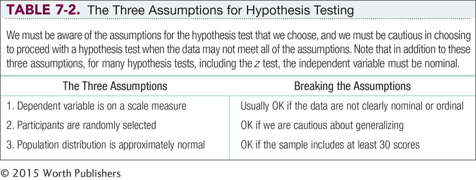
These three statistical assumptions represent the ideal conditions and are more likely to produce valid research. Meeting the assumptions improves the quality of research, but not meeting the assumptions doesn’t necessarily invalidate research.
The Six Steps of Hypothesis Testing
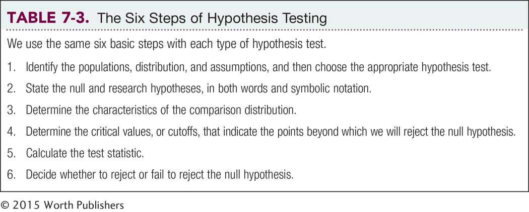
Hypothesis testing can be broken down into six standard steps.
Step 1: Identify the populations, comparison distribution, and assumptions.
When we first approach hypothesis testing, we consider the characteristics of the data in order to determine the distribution to which we will compare the sample. First, we state the populations represented by the groups to be compared. Then we identify the comparison distribution (e.g., a distribution of means). Finally, we review the assumptions of hypothesis testing. The information we gather in this step helps us to choose the appropriate hypothesis test (Appendix E, Figure E-1, provides a quick guide for choosing the appropriate test).
Step 2: State the null and research hypotheses.
Hypotheses are about populations, not about samples. The null hypothesis is usually the “boring” one that posits no change or no difference between groups. The research hypothesis is usually the “exciting” one that posits, for example, that a given intervention will lead to a change or a difference—
Step 3: Determine the characteristics of the comparison distribution.
State the relevant characteristics of the comparison distribution (the distribution based on the null hypothesis). In a later step, we will compare data from the sample (or samples) to the comparison distribution to determine how extreme the sample data are. For z tests, we will determine the mean and standard error of the comparison distribution. These numbers describe the distribution represented by the null hypothesis and will be used when we calculate the test statistic.
Step 4: Determine the critical values, or cutoffs.
A critical value is a test statistic value beyond which we reject the null hypothesis; often called a cutoff.
The critical values, or cutoffs, of the comparison distribution indicate how extreme the data must be, in terms of the z statistic, to reject the null hypothesis. Often called simply cutoffs, these numbers are more formally called critical values, the test statistic values beyond which we reject the null hypothesis. In most cases, we determine two cutoffs: one for extreme samples below the mean and one for extreme samples above the mean.
The critical region is the area in the tails of the comparison distribution in which the null hypothesis can be rejected.
The probability used to determine the critical values, or cutoffs, in hypothesis testing is a p level (often called alpha).
The critical values, or cutoffs, are based on a somewhat arbitrary standard—
Step 5: Calculate the test statistic.
We use the information from step 3 to calculate the test statistic, in this case the z statistic. We can then directly compare the test statistic to the critical values to determine whether the sample is extreme enough to warrant rejecting the null hypothesis.
Step 6: Make a decision.
Using the statistical evidence, we can now decide whether to reject or fail to reject the null hypothesis. Based on the available evidence, we either reject the null hypothesis if the test statistic is beyond the cutoffs, or we fail to reject the null hypothesis if the test statistic is not beyond the cutoffs.
These six steps of hypothesis testing are summarized in Table 7-3.
A finding is statistically significant if the data differ from what we would expect by chance if there were, in fact, no actual difference.
Language Alert! When we reject the null hypothesis, we often refer to the results as “statistically significant.” A finding is statistically significant if the data differ from what we would expect by chance if there were, in fact, no actual difference. The word significant is another one of those statistical terms with a very particular meaning. The phrase statistically significant does not necessarily mean that the finding is important or meaningful. A small difference between means could be statistically significant but not practically significant or important.
CHECK YOUR LEARNING
| Reviewing the Concepts |
|
|
| Clarifying the Concepts | 7- |
Explain the three assumptions made for most parametric hypothesis tests. |
| 7- |
How do critical values help us to make a decision about the hypothesis? | |
| Calculating the Statistics | 7- |
If a researcher always sets the critical region as 8% of the distribution, and the null hypothesis is true, how often will he reject the null hypothesis if the null hypothesis is true? |
| 7- |
Rewrite each of these percentages as a probability, or p level: | |
|
||
| Applying the Concepts | 7- |
For each of the following scenarios, state whether each of the three basic assumptions for parametric hypothesis tests is met. Explain your answers and label the three assumptions (1) through (3). |
|
Solutions to these Check Your Learning questions can be found in Appendix D.