8-1: We can use a sample to calculate a point estimate—one plausible number, such as a mean—for the population. More realistically, we also can use a sample to calculate an interval estimate—a range of plausible numbers, such as a range of means—for the population.

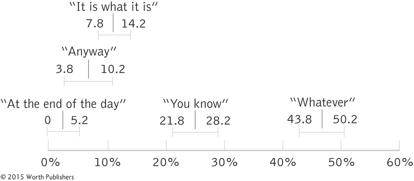
For example, a Marist poll asked 938 adult respondents in the United States to select from five choices the word or phrase that they found “most annoying in conversation” (http://maristpoll.marist.edu/-107-whatever-takes-top-honors-as-most-annoying/). “Whatever” was chosen by 47% of respondents, ahead of “you know” (25%), “it is what it is” (11%), “anyway” (7%), and “at the end of the day” (2%). The margin of error was reported to be ±3.2% (plus or minus 3.2%).

Because 47 − 3.2 = 43.8 and 47 + 3.2 = 50.2, the interval estimate for “whatever” is 43.8% to 50.2% (Figure 8-2). Interval estimates provide a range of plausible values, not just one statistic.

Pay attention to whether the interval estimates overlap. “You know” came in second, with 25%, giving an interval estimate of 21.8% to 28.2%. There’s no overlap with the first-place word, a strong indication that “whatever” really was most annoying in the population as well as in the sample. However, if “you know” had received 42% of the vote, it would have placed only 5% behind “whatever,” and it would have had an interval estimate of 38.8% to 45.2%. This range would have overlapped with the one for “whatever” (43.8% to 50.2%), an indication that both expressions could plausibly have been equally annoying in the population.

Language Alert! The terms “margin of error,” “interval estimate,” and “confidence interval” all represent the same idea. Specifically, a confidence interval is an interval estimate based on a sample statistic; it includes the population mean a certain percentage of the time if the same population is sampled from repeatedly. (Note: We are not saying that we are confident that the population mean falls in the interval; we are merely saying that we expect to find the population mean within a certain interval a certain percentage of the time—usually 95%—when we conduct this same study with the same sample size.)

The confidence interval is centered around the mean of the sample. A 95% confidence level is most commonly used, indicating the 95% that falls between the two tails (i.e., 100% − 5% = 95%). Note the terms used here: The confidence level is 95%, but the confidence interval is the range between the two values that surround the sample mean.

We already conducted hypothesis testing in Example 7.5 in Chapter 7 for a study on calories consumed by patrons of different Starbucks stores that either did or did not post the calories on their menus (Bollinger, Leslie, & Sorensen, 2010). Here is how confidence intervals can help us listen more closely to the story these data tell. The population mean was 247 calories, and we considered 201 to be the population standard deviation. The 1000 people in the sample consumed a mean of 232 calories. When we conducted hypothesis testing, we centered the curve around the mean according to the null hypothesis, the population mean of 247. We determined critical values based on this mean and compared the sample mean to these cutoffs. The test statistic (−2.36) was beyond the critical z statistic, so we rejected the null hypothesis. The data led us to conclude that people going to those Starbucks that posted calories consumed fewer calories, on average, than people going to those Starbucks that did not post calories.

189

There are several steps to calculating a confidence interval.

STEP 1: Draw a picture of a distribution that will include the confidence interval.

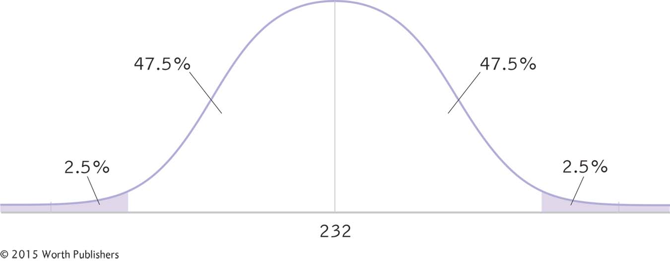
We draw a normal curve (Figure 8-3) that has the sample mean, 232, at its center, instead of the population mean, 247.

STEP 2: Indicate the bounds of the confidence interval on the drawing.

We draw a vertical line from the mean to the top of the curve. For a 95% confidence interval, we also draw two small vertical lines to indicate the middle 95% of the normal curve (2.5% in each tail, for a total of 5%).

The curve is symmetric, so half of the 95% falls above and half falls below the mean. Half of 95 is 47.5, so we write 47.5% in the segments on either side of the mean. In the tails beyond the two lines that indicate the end of the middle 95%, we also write the appropriate percentages. You can see these percentages in Figure 8-3.

STEP 3: Determine the z statistics that fall at each line marking the middle 95%.

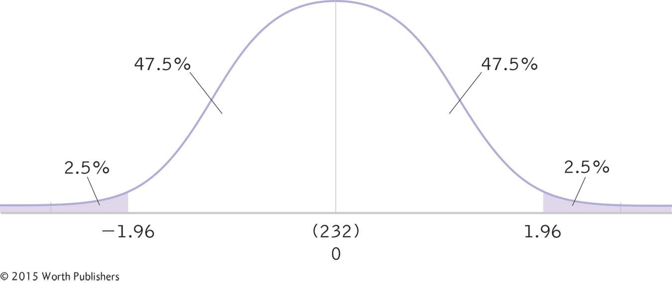
To do this, we turn back to the versatile z table in Appendix B. The percentage between the mean and each of the z scores is 47.5%. When we look up this percentage in the z table, we find a z statistic of 1.96. (Note that this is identical to the cutoffs for the z test; this will always be the case because the p level of 0.05 corresponds to a confidence level of 95%.) We can now add the z statistics of −1.96 and 1.96 to the curve, as seen in Figure 8-4.

STEP 4: Turn the z statistics back into raw means.

We use the formula for this conversion, but first we identify the appropriate mean and standard deviation. There are two important points to remember. First, we center the interval around the sample mean (not the population mean). So we use the sample mean of 232 in the calculations. Second, because we have a sample mean (rather than an individual score), we use a distribution of means. So we calculate standard error as the measure of spread:

190

Notice that this is the same standard error that we calculated in Example 7.5 in Chapter 7 when we conducted a hypothesis test.

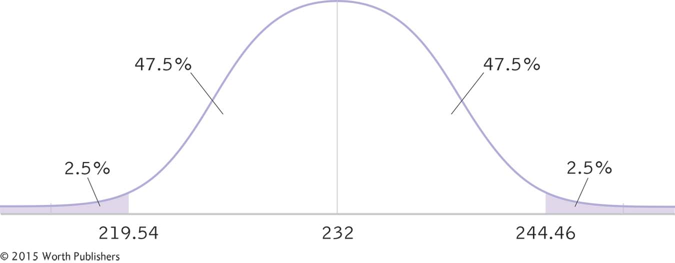
Using this mean and standard error, we calculate the raw mean at each end of the confidence interval, and add them to the curve, as in Figure 8-5:

M_lower = −z(σ_M) + M_sample = −1.96(6.356) + 232 = 219.54

M_upper = z(σ_M) + M_sample = 1.96(6.356) + 232 = 244.46

The 95% confidence interval, reported in brackets as is typical, is [219.54, 244.46].

STEP 5: Check that the confidence interval makes sense.

The sample mean should fall exactly in the middle of the two ends of the interval.

219.54 − 232 = −12.46 and 244.46 − 232 = 12.46

We have a match. The confidence interval ranges from 12.46 below the sample mean to 12.46 above the sample mean. We can think of this number, 12.46, as the margin of error.

To recap the steps for the creation of a confidence interval for a z statistic:

If we were to sample 1000 customers at the Starbucks that post calories on their menus from the same population over and over, the 95% confidence interval would include the population mean 95% of the time. Note that the population mean for customers at the Starbucks that do not post calories, 247, falls outside of this interval. So, it is not plausible that the sample of customers at Starbucks that post calories comes from the population according to the null hypothesis—customers at Starbucks that do not post calories. The conclusions from both the z test and the confidence interval are the same, but the confidence interval gives us more information—an interval estimate, not just a point estimate. Moreover, there is some evidence that reporting confidence intervals instead of the results of hypothesis testing can lead to more accurate interpretations of the findings (Coulson, Healey, Fidler, & Cumming, 2010).

Solutions to these Check Your Learning questions can be found in Appendix D.