8.3 Statistical Power
The effect size statistic tells us that the public controversy over gender differences in mathematical ability was justified: The observed gender differences had no practical importance. Calculating statistical power is another way to limit such controversies from developing in the first place.
Statistical power is a measure of the likelihood that we will reject the null hypothesis, given that the null hypothesis is false.
Power is a word that statisticians use in a very specific way. Statistical power is a measure of the likelihood that we will reject the null hypothesis, given that the null hypothesis is false. In other words, statistical power is the probability that we will reject the null hypothesis when we should reject the null hypothesis—

MASTERING THE CONCEPT
8-
The calculation of statistical power ranges from a probability of 0.00 to a probability of 1.00 (or from 0% to 100%). Statisticians have historically used a probability of 0.80 as the minimum for conducting a study. If we have an 80% chance of correctly rejecting the null hypothesis, then it is appropriate to conduct the study. Let’s look at statistical power for a one-
The Importance of Statistical Power
To understand statistical power, we need to consider several characteristics of the two populations of interest: the population we believe the sample represents (population 1) and the population to which we’re comparing the sample (population 2). We represent these two populations visually as two overlapping curves. Let’s consider a variation on an example from Chapter 4—a study aimed at determining whether an intervention changes the mean number of sessions attended at university counseling centers (Hatchett, 2003).
EXAMPLE 8.5
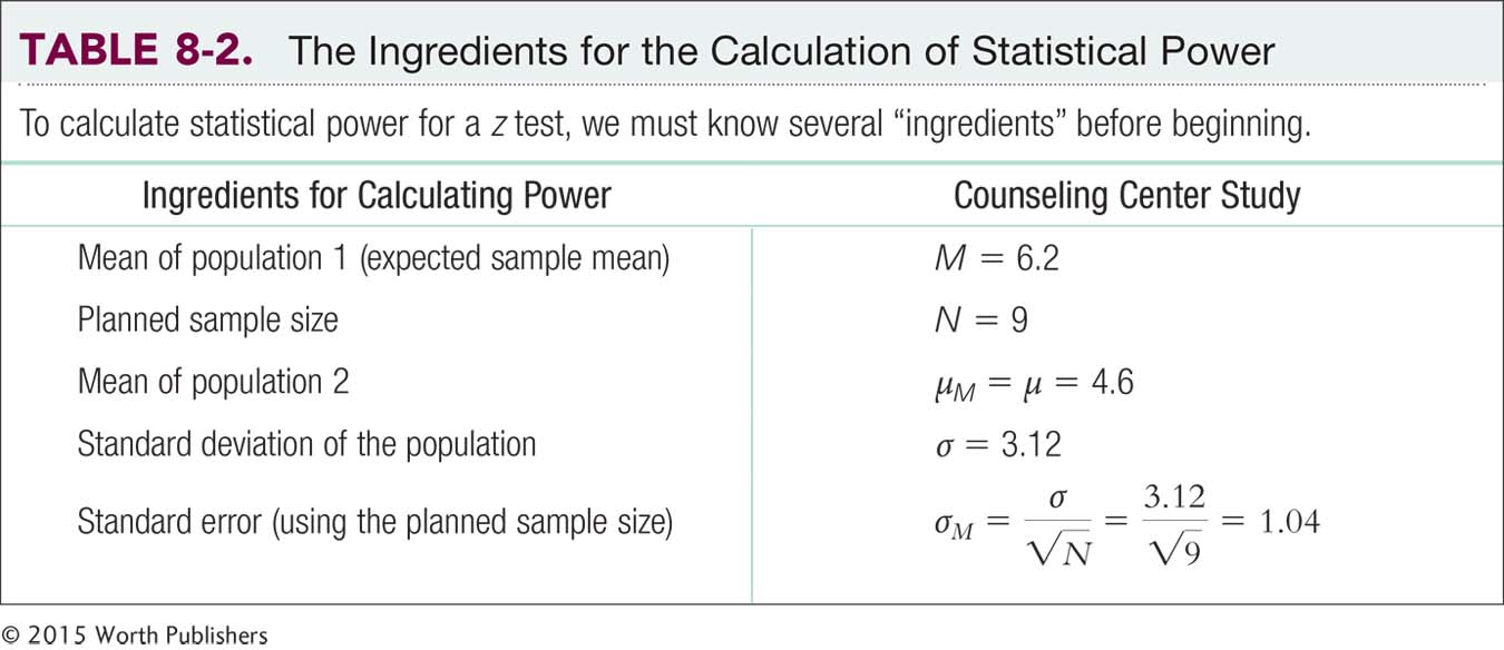
STEP 1: Determine the information needed to calculate statistical power—
In this example, let’s say that we hypothesize that a sample of 9 counseling center students will have a mean number of 6.2 sessions after the intervention. The population mean number of sessions attended is 4.6, with a population standard deviation of 3.12. The sample mean of 6.2 is an increase of 1.6 over the population mean, the equivalent of a Cohen’s d of about 0.5, a medium effect. Because we have a sample of 9, we need to convert the standard deviation to standard error; to do this, we divide the standard deviation by the square root of the sample size and find that standard error is 1.04. The numbers needed to calculate statistical power are summarized in Table 8-2. We call the population from which the sample comes “population 1” and the population for which we know the mean “population 2.”
You might wonder how we came up with the hypothesized sample mean, 6.2. We never know, particularly prior to a study, what the actual effect will be. Researchers typically estimate the mean of population 1 by examining the existing research literature or by deciding how large an effect size would be needed to make the study worthwhile (Murphy & Myors, 2004). Some statisticians recommend erring on the side of using smaller, more conservative effect sizes in power calculations, and others recommend calculating power for a range of effect sizes (Gelman & Carlin, 2014; McShane and Böckenholt, 2014). In this case, we hypothesized a medium effect—
STEP 2: Determine a critical value in terms of the z distribution and the raw mean so that statistical power can be calculated.
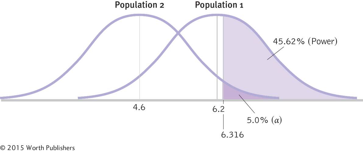
For this example, the distribution of means for population 1, centered around 6.2, and the distribution of means for population 2, centered around 4.6, are shown in Figure 8-9. This figure also shows the critical value for a one-
M = 1.65(1.04) + 4.6 = 6.316
Statistical Power: The Whole Picture
Now we can visualize statistical power in the context of two populations. Statistical power is the percentage of the distribution of means for population 1 that is above the cutoff. Here the statistical power is 45.62%. Alpha (α) is the percentage of the distribution of means for population 2 that is above the cutoff; alpha is set by the researcher and is usually 0.05, or 5%.
The p level is shaded in dark purple and marked as 5.0% (α), the percentage version of a proportion of 0.05. The critical value of 6.316 marks off the upper 5% of the distribution based on the null hypothesis, for population 2.
This critical value, 6.316, has the same meaning as it did in hypothesis testing. If the test statistic for a sample falls above this cutoff, then we reject the null hypothesis. Notice that the mean we estimated for population 1 does not fall above the cutoff. If the actual difference between the two populations is what we expect, then we can already see that there is a good chance we will not reject the null hypothesis with a sample size of 9. This indicates that we might not have enough statistical power.
STEP 3: Calculate the statistical power—
The proportion of the curve above the critical value, shaded in light purple in Figure 8-9, is statistical power, which can be calculated with the use of the z table. Remember, statistical power is the chance that we will reject the null hypothesis if we should reject the null hypothesis.
Statistical power in this case is the percentage of the distribution of means for population 1 (the distribution centered around 6.2) that falls above the critical value of 6.316. We convert this critical value to a z statistic based on the hypothesized mean of 6.2.
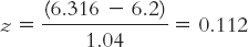
We look up this z statistic on the z table to determine the percentage above a z statistic of 0.112. That percentage, the area shaded in light purple in Figure 8-9, is 45.62%.
From Figure 8-9, we see the critical value as determined in reference to population 2; in raw score form, it is 6.316. We see that the percentage of the distribution of means for population 2 that falls above 6.316 is 0.05, or 5%, the usual p level that was introduced in Chapter 7. The p level is the chance of making a Type I error. When we turn to the distribution of means for population 1, the percentage above that same cutoff is the statistical power. Given that population 1 exists, 45.62% of the time that we select a sample of size 9 from this population, we will be able to reject the null hypothesis. This is far below the 80% considered adequate, and we would be wise to increase the sample size.
On a practical level, statistical power calculations tell researchers how many participants are needed to conduct a study whose findings we can trust. Remember, however, that statistical power is based to some degree on hypothetical information, and it is just an estimate. We turn next to several factors that affect statistical power.
Five Factors That Affect Statistical Power
Here are five ways to increase the power of a statistical test, from the easiest to the most difficult:
Increase alpha. Increasing alpha is like changing the rules by widening the goal posts in football or the goal in soccer. In Figure 8-10, we see how statistical power increases when we increase a p level of 0.05 (see Figure 8-10a) to 0.10 (see Figure 8-10b). This has the side effect of increasing the probability of a Type I error from 5% to 10%, however, so researchers rarely choose to increase statistical power in this manner.
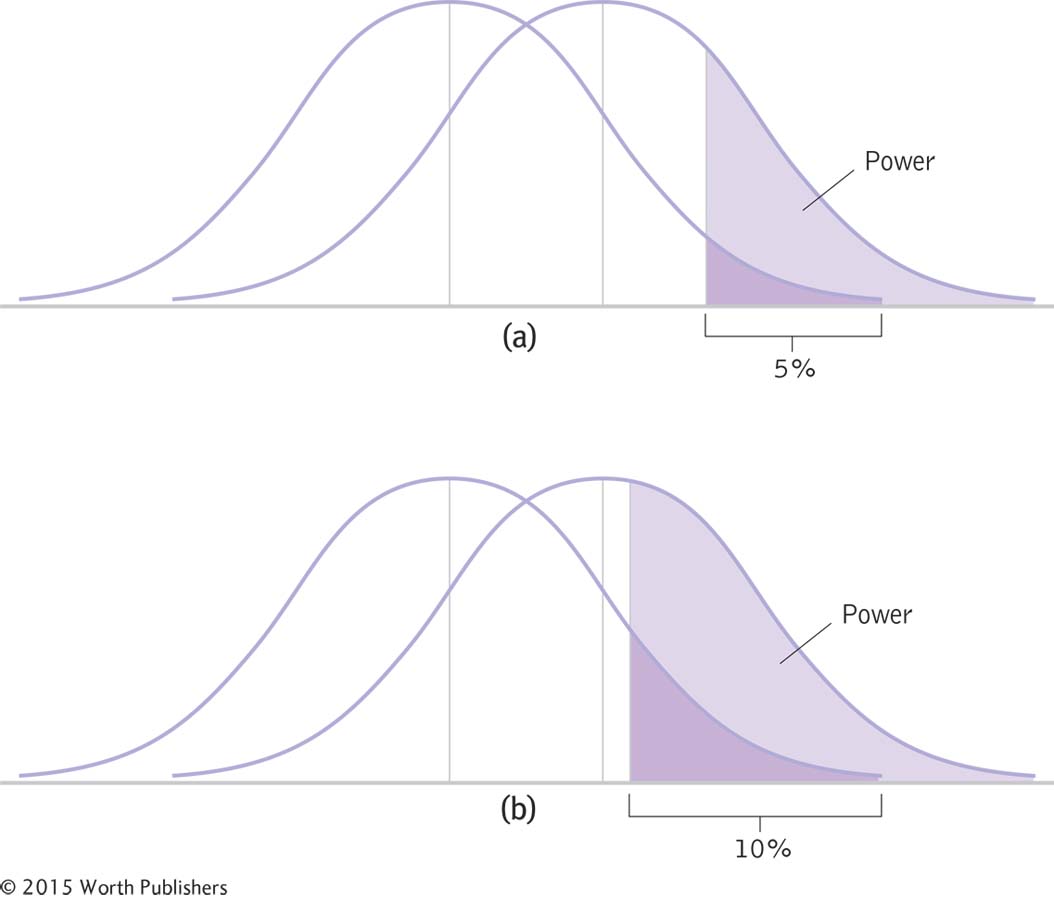 Figure 8.11: FIGURE 8-
10
Increasing Alpha
As we increase alpha from the standard of 0.05 to a larger level, such as 0.10, statistical power increases. Because this also increases the probability of a Type I error, this is not usually a good method for increasing statistical power.Turn a two-
tailed hypothesis into a one- tailed hypothesis. We have been using a simpler one- tailed test, which provides more statistical power. However, researchers usually begin with the more conservative two- tailed test. In Figure 8-11, we see the difference between the less powerful two- tailed test (part (a)) and the more powerful one- tailed test (part (b)). The curves in part (a), with a two- tailed test, show less statistical power than do the curves in part (b). However, it is usually best to be conservative and use a two- tailed test. Page 202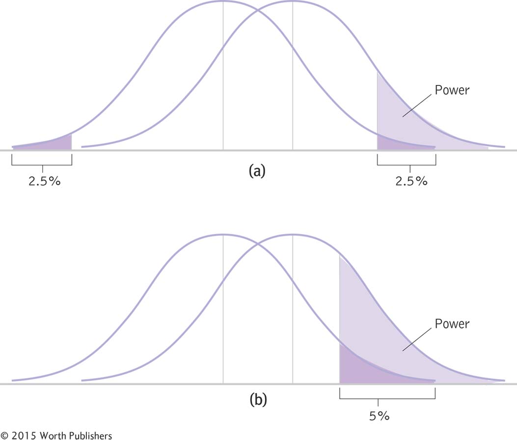 Figure 8.12: FIGURE 8-
11
Two-Tailed Versus One- Tailed Tests
A two-tailed test divides alpha into two tails. When we use a one- tailed test, putting the entire alpha into just one tail, we increase the chances of rejecting the null hypothesis, which translates into an increase in statistical power. Increase N. As we demonstrated earlier in this chapter, increasing sample size leads to an increase in the test statistic, making it easier to reject the null hypothesis. The curves in Figure 8-12a represent a small sample size; those in Figure 8-12b represent a larger sample size. The curves are narrower in part (b) than in part (a) because a larger sample size means smaller standard error. We have direct control over sample size, so simply increasing N is often an easy way to increase statistical power.
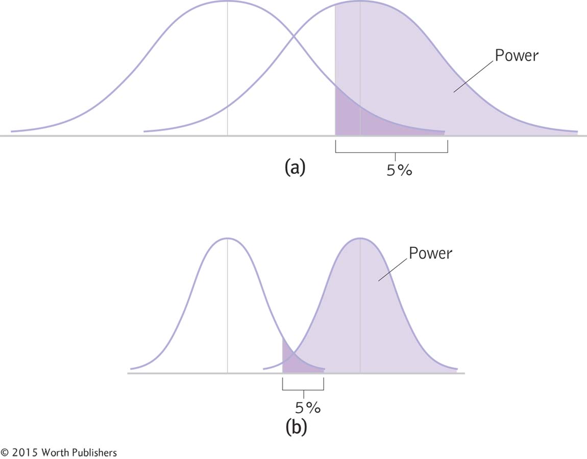 Figure 8.13: FIGURE 8-
12
Increasing Sample Size or Decreasing Standard Deviation
As sample size increases, from part (a) to part (b), the distributions of means become more narrow and there is less overlap. Less overlap means more statistical power. The same effect occurs when we decrease standard deviation. As standard deviation decreases, also reflected from part (a) to part (b), the curves are narrower and there is less overlap—and more statistical power. - Page 203
Exaggerate the mean difference between levels of the independent variable. As seen in Figure 8-13, the mean of population 2 is farther from the mean of population 1 in part (b) than it is in part (a). The difference between means is not easily changed, but it can be done. For instance, if we were studying the effectiveness of group therapy for social phobia, we could increase the length of therapy from 12 weeks to 6 months. It is possible that a longer program might lead to a larger change in means than would the shorter program.
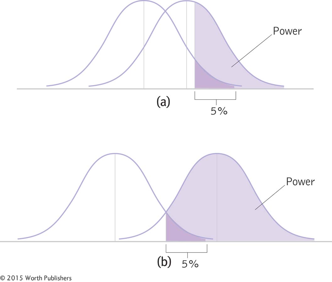 Figure 8.14: FIGURE 8-
13
Increasing the Difference Between the Means
As the difference between means becomes larger, there is less overlap between curves. Here, the lower pair of curves has less overlap than the upper pair. Less overlap means more statistical power. Decrease standard deviation. We see the same effect on statistical power if we find a way to decrease the standard deviation as when we increase sample size. Look again at Figure 8-12, which reflects an increase in sample size. The curves can become narrower not just because the denominator of the standard error calculation is larger, but also because the numerator is smaller. When standard deviation is smaller, standard error is smaller, and the curves are narrower. We can reduce standard deviation in two ways: (1) by using reliable measures from the beginning of the study, thus reducing error, or (2) by sampling from a more homogeneous group in which participants’ responses are more likely to be similar to begin with.
Because statistical power is affected by so many variables, it is important to consider when reading about research. Always ask whether there was sufficient statistical power to detect a real finding. Most importantly, were there enough participants in the sample?
The most practical way to increase statistical power for many behavioral studies is by adding more participants to your study. You can estimate how many participants you need for your particular research design by referring to a table such as that in Jacob Cohen’s (1992) article, “A Power Primer.” You can also download the free software G*Power, available for Mac or PC (Erdfelder, Faul, & Buchner, 1996; search online for G*Power or find the link on the Web site for this book).
Statistical power calculators like G*Power are versatile tools that are typically used in one of two ways. First, we can calculate power after conducting a study from several pieces of information. For most electronic power calculators, including G*Power, we determine power by inputting the effect size and sample size along with some of the information that we outlined earlier in Table 8-2. We calculate power after determining effect size and other characteristics, so G*Power refers to these calculations as post hoc, which means “after the fact.” Second, we can use them in reverse, before conducting a study, by calculating the sample size necessary to achieve a given level of power. In this case, we use a power calculator to determine the sample size necessary to achieve the statistical power that we want before we conduct the study. G*Power refers to such calculations as a priori, which means “prior to.”
The controversy over the 1980 Benbow and Stanley study of gender differences in mathematical ability demonstrates why it is important to go beyond hypothesis testing. The study used 10,000 participants, so it had plenty of statistical power. That means we can trust that the statistically significant difference they found was real. But the effect size informed us that this statistically significant difference was trivial. Combining all four ways of analyzing data (hypothesis testing, confidence intervals, effect size, and power analysis) helps us listen to the data story with all of its wonderful nuances and suggestions for future research.
CHECK YOUR LEARNING
| Reviewing the Concepts |
|
|
| Clarifying the Concepts | 8- |
What are three ways to increase statistical power? |
| Calculating the Statistics | 8- |
Check Your Learning 8- |
| Applying the Concepts | 8- |
Refer to Check Your Learning 8-
|
Solutions to these Check Your Learning questions can be found in Appendix D.