nolanessentials3e

9.3 The Paired-Samples t Test

As we learned in the chapter opening, researchers found that weight gain over the holidays is far less than what folk wisdom had suggested. Guess what? The dreaded “freshman 15” also appears to be a myth. One study found that male university students gained an average of 3.5 pounds between the beginning of the fall semester and November, and female students gained an average of 4.0 pounds (Holm-Denoma, Joiner, Vohs, & Heatherton, 2008). We can use the paired-samples t test to make before-and-after comparisons.

227

The paired-samples t test is used to compare two means for a within-groups design, a situation in which every participant is in both samples; also called a dependent-samples t test

The paired-samples t test (also called the dependent-samples t test) is used to compare two means for a within-groups design, a situation in which every participant is in both samples. The paired-samples t test can be used to analyze the data from many studies. For example, if a participant is in both conditions (such as a memory task before ingesting a caffeinated beverage and again after ingesting a non-caffeinated beverage), then her score in one depends on her score in the other.

The steps for the paired-samples t test are almost the same as those for the single-sample t test. The major difference in the paired-samples t test is that we must create difference scores for every participant. Because we’ll be working with difference scores, we need to learn about a new distribution—a distribution of the means of these difference scores, or a distribution of mean differences.

Before and After Don’t be fooled by one dramatic before-and-after story! Before you start a potentially dangerous diet or have an expensive surgical procedure, ask for the results of an independently conducted paired-samples t test.

Distributions of Mean Differences

We already learned about a distribution of scores and a distribution of means. Now we need to develop a distribution of mean differences for the pre- and postholiday weight data. Our goal is to establish a distribution that specifies the null hypothesis for a within-groups design.

Imagine that many college students’ weights were measured before and after the winter holidays and written on individual cards. We begin by gathering data from a sample of three people from among this population of many college students. There are two cards for each person in the population, on which weights are listed—one before the holidays and one after the holidays. We have one pair of cards for each student in the population (which is why one name for this test is the paired-samples t test). Let’s walk through the steps to create a distribution of mean differences.

228

Step 1: Randomly choose three pairs of cards, replacing each pair of cards before randomly selecting the next.

Step 2: For each pair, calculate a difference score by subtracting the first weight from the second weight.

Step 3: Calculate the mean of the differences in weights for these three people. Then complete these three steps again. Randomly choose another three people from the population of many college students, calculate their difference scores, and calculate the mean of the three difference scores. And then complete these three steps again, and again, and again.

Let’s walk through these steps once again, using an example.

Step 1: We randomly select one pair of cards and find that the first student weighed 140 pounds before the holidays and 144 pounds after the holidays. We replace those cards and randomly select another pair; the second student had before and after scores of 126 and 124, respectively. We replace those cards and randomly select another pair; the third student had before and after scores of 168 and 168, respectively.

Step 2: For the first student, the difference between weights, subtracting the before score from the after score, is 144 − 140 = 4. She gained 4 pounds. For the second student, the difference between weights is 124 − 126 = −2. He lost 2 pounds. For the third student, the difference between weights is 168 − 168 = 0. Her weight did not change.

Step 3: The mean of these three difference scores (4, −2, 0) is 0.667. The mean change in weight is a gain of 0.667 pounds.

We would then choose three more students and calculate the mean of their difference scores. Eventually, we would have many mean differences to plot on a curve of mean differences—some positive, some negative, and some right at 0.

But this would only be the beginning of what this distribution of mean differences would look like. If we were to calculate the whole distribution of mean differences, then we would do this an uncountable number of times. When the authors of this book calculated 30 mean differences for pairs of weights, we got the distribution in Figure 9-7. If no mean difference is found when comparing weights from before and after the holidays, as with the data we used to create Figure 9-7, the distribution would center around 0. According to the null hypothesis, we would expect no mean difference in weight—or a mean difference of 0—from before the holidays to after the holidays.

Figure 9.8: FIGURE 9-7
Creating a Distribution of Mean Differences

Figure 9.8: This distribution is one of many that could be created by pulling 30 mean differences—the average of three differences between pairs of weights, pulled one at a time from a population of pairs of weights—one preholiday and one postholiday. The population used here is one based on the null hypothesis—that there is no average difference in weight from before the holidays to after the holidays.

229

The Six Steps of the Paired-Samples t Test

In a paired-samples t test, each participant has two scores—one in each condition. When we conduct a paired-samples t test, we write the pairs of scores in two columns, side by side next to the same participant. We then subtract each score in one column from its paired score in the other column to create difference scores. Ideally, a positive difference score indicates an increase, and a negative difference score indicates a decrease. Typically, we subtract the first score from the second so that the difference scores match this logic. We will now walk through the six steps of hypothesis testing for the paired-samples t test.

Large Monitors and Productivity Does a large monitor increase your productivity? Microsoft researchers and cognitive psychologists (Czerwinski et al., 2003) reported a 9% increase in productivity when research volunteers used a large 42-inch display versus a 15-inch display. Every participant used both displays and thus was in both samples. A paired-samples t test is the appropriate hypothesis test for this two-group design.

EXAMPLE 9.9

Let’s use an example from the software industry (which employs social scientists to improve the ways in which people interact with their products). For example, behavioral scientists at Microsoft studied how 15 volunteers performed on a set of tasks under two conditions—while using a 15-inch computer monitor and while using a 42-inch monitor (Czerwinski et al., 2003), the latter of which allows the user to have multiple programs in view at the same time.

Here are five participants’ fictional data, which reflect the actual means reported by the researchers. Note that a smaller number is good—it indicates a faster time. The first person completed the tasks on the small monitor in 122 seconds and on the large monitor in 111 seconds; the second person in 131 and 116; the third in 127 and 113; the fourth in 123 and 119; and the fifth in 132 and 121.

STEP 1: Identify the populations, distribution, and assumptions.

MASTERING THE CONCEPT

9-5: The steps for the paired-samples t test are similar to those for the single-sample t test. The main difference is that for the paired-samples t test, we compare the sample mean difference between scores to the mean difference for the population according to the null hypothesis, rather than comparing the sample mean of individual scores to the population mean according to the null hypothesis, as we do when conducting a single-sample t test.

The paired-samples t test is like the single-sample t test in that we analyze a single sample of scores. For the paired-samples t test, however, we analyze difference scores. For the paired-samples t test, one population is reflected by each condition, but the comparison distribution is a distribution of mean difference scores (rather than a distribution of means). The comparison distribution is based on the null hypothesis that posits no mean difference. So the mean of the comparison distribution is 0. For the paired-samples t test, the three assumptions are the same as for the single-sample t test.

Summary: Population 1: People performing tasks using a 15-inch monitor. Population 2: People performing tasks using a 42-inch monitor.

The comparison distribution is a distribution of mean difference scores based on the null hypothesis. The hypothesis test is a paired-samples t test because we have two samples of scores and a within-groups design.

230

This study meets one of the three assumptions and may meet the other two: (1) The dependent variable is time, which is scale. (2) The participants were not randomly selected, however, so we must be cautious with respect to generalizing the findings. (3) We do not know whether the population is normally distributed, and there are not at least 30 participants. However, the data from this sample do not suggest a skewed distribution.

STEP 2: State the null and research hypotheses.

This step is identical to that for the single-sample t test.

Summary: Null hypothesis: People who use a 15-inch screen will complete a set of tasks in the same amount of time, on average, as people who use a 42-inch screen—H₀: µ₁ = µ₂. Research hypothesis: People who use a 15-inch screen will complete a set of tasks in a different amount of time, on average, than people who use a 42-inch screen—H₁: µ₁ ≠ µ₂.

STEP 3: Determine the characteristics of the comparison distribution.

This step is similar to that for the single-sample t test. We determine the appropriate mean and standard error of the comparison distribution—the distribution based on the null hypothesis. With the paired-samples t test, however, we have a sample of difference scores and a comparison distribution of mean differences (instead of a sample of individual scores and a comparison distribution of means). According to the null hypothesis, there is no difference. So the mean of the comparison distribution is always 0, as long as the null hypothesis posits no difference.

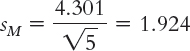
For the paired-samples t test, standard error is calculated exactly as it is calculated for the single-sample t test, only we use the difference scores rather than the scores in each condition. To get the difference scores in the current example, we want to know what happens when we go from the control condition (small screen) to the experimental condition (large screen), so we subtract the first score from the second score. This means that a negative difference indicates a decrease in time when the screen goes from small to large. (The test statistic will be the same if we reverse the order in which we subtract, but the sign will change.)

Summary: µ_M = 0; s_M = 1.924

Calculations: (Notice that we crossed out the original scores once we created the column of difference scores. We did this to remind ourselves that all remaining calculations involve the differences scores, not the original scores.)

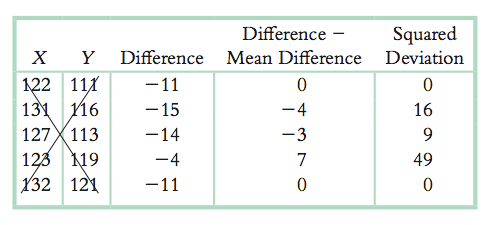
The mean of the difference scores is:

M_difference = −11

The numerator is the sum of squares, SS (which we learned about in Chapter 4):

SS = 0 + 16 + 9 + 49 + 0 = 74

231

The standard deviation, s, is:

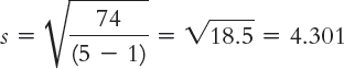
The standard error, s_M, is:

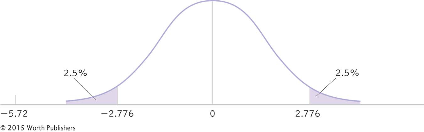
STEP 4: Determine the critical values, or cutoffs.

This step is the same as that for the single-sample t test, except that the degrees of freedom is the number of participants (not the number of scores) minus 1.

Summary: df = N − 1 = 5 − 1 = 4

The critical values, based on a two-tailed test and a p level of 0.05, are −2.776 and 2.776, as seen in the curve in Figure 9-8.

Figure 9.9: FIGURE 9-8
Determining Cutoffs for a Paired-Samples t Test

Figure 9.9: We typically determine critical values in terms of t statistics rather than means of raw scores so that we can easily determine whether the test statistic is beyond one of the cutoffs.

STEP 5: Calculate the test statistic.

This step is identical to that for the single-sample t test, except that we use means of difference scores instead of means of individual scores. We subtract the mean difference score according to the null hypothesis, 0, from the mean difference score calculated for the sample. We then divide by standard error.

Summary: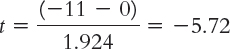

STEP 6: Make a decision.

This step is identical to that for the single-sample t test.

Summary: Reject the null hypothesis. When we examine the means (M_X = 127; M_Y = 116), it appears that, on average, people perform faster when using a 42-inch monitor than when using a 15-inch monitor (as shown by the curve in Figure 9-9).

Figure 9.10: FIGURE 9-9
Making a Decision

Figure 9.10: To decide whether to reject the null hypothesis, we compare the test statistic to the critical values. In this figure, the test statistic, −5.72, is beyond the cutoff of −2.776, so we can reject the null hypothesis.

232

The statistics, as reported in a journal article, follow the same APA format as for a single-sample t test. (Note: Unless we use software, we can only indicate whether the p value is less than or greater than the cutoff p level of 0.05.) In the current example, the statistics would read:

t(4) = −5.72, p < 0.05

We also include the means and the standard deviations for the two samples. We calculated the means in step 6 of hypothesis testing, but we would also have to calculate the standard deviations for the two samples to report them.

The researchers note that the faster time with the large display might not seem much faster but that, in their research, they have had great difficulty identifying any factors that lead to faster times (Czerwinski et al., 2003). Based on their previous research, therefore, this is an impressive difference.

Calculating a Confidence Interval for a Paired-Samples t Test

MASTERING THE CONCEPT

9-6: As we can with a z test and a single-sample t test, we can calculate a confidence interval and an effect size for a paired-samples t test.

The APA encourages the use of confidence intervals and effect sizes (as with the z test and the single-sample t test) for paired-samples t tests. We’ll calculate both the confidence interval and the effect size for the example of productivity with small versus large computer monitors.

EXAMPLE 9.10

Let’s start by determining the confidence interval for the productivity example. First, let’s recap the information we need. The population mean difference according to the null hypothesis was 0, and we used the sample to estimate the population standard deviation to be 4.301 and the standard error to be 1.924. The five participants in the study sample had a mean difference of −11. We will calculate the 95% confidence interval around the sample mean difference of −11.

STEP 1: Draw a picture of a t distribution that includes the confidence interval.

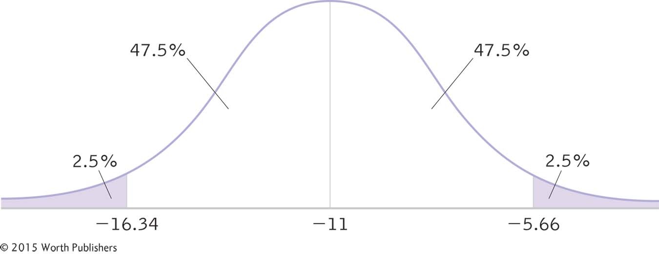
We draw a normal curve (Figure 9-10) that has the sample mean difference, −11, at its center instead of the population mean difference, 0.

Figure 9.11: FIGURE 9-10
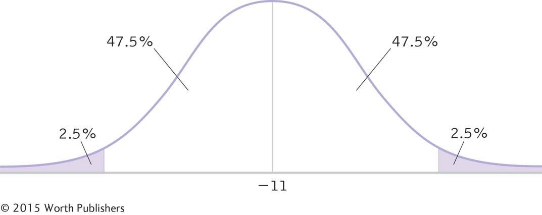
A 95% Confidence Interval for a Paired-Samples t Test, Part I

Figure 9.11: We start the confidence interval for a distribution of mean differences by drawing a curve with the sample mean difference, −11, in the center.

STEP 2: Indicate the bounds of the confidence interval on the drawing.

As before, 47.5% fall on each side of the mean between the mean and the cutoff, and 2.5% fall in each tail.

233

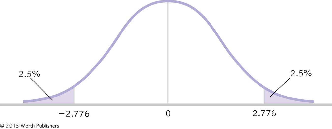
STEP 3: Add the critical t statistics to the curve.

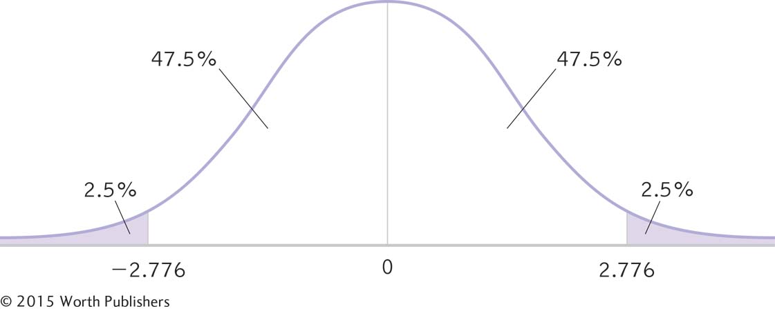
For a two-tailed test with a p level of 0.05 and 4 df, the critical values are −2.776 and 2.776, as seen in Figure 9-11.

Figure 9.12: FIGURE 9-11
A 95% Confidence Interval for a Paired-Samples t Test, Part II

Figure 9.12: The next step in calculating a confidence interval for mean differences is identifying the t statistics that indicate each end of the interval. Because the curve is symmetric, the t statistics have the same magnitude—one is negative, −2.776, and one is positive, 2.776.

STEP 4: Convert the critical t statistics back into raw mean differences.

As we do with other confidence intervals, we use the sample mean difference (−11) in the calculations and the standard error (1.924) as the measure of spread. We use the same formulas as for the single-sample t test, recalling that these means and standard errors are calculated from differences between two scores for each participant. We add these raw mean differences to the curve in Figure 9-12.

Figure 9.13: FIGURE 9-12
A 95% Confidence Interval for a Paired-Samples t Test, Part III

Figure 9.13: The final step in calculating a confidence interval for mean differences is converting the t statistics that indicate each end of the interval to raw mean differences, −16.34 and −5.66.

M_lower = −t(s_M) + M_sample = −2.776(1.924) + (−11) =−16.34

M_upper = t(s_M) + M_sample = 2.776(1.924) + (−11) =−5.66

The 95% confidence interval, reported in brackets as is typical, is [−16.34, −5.66].

STEP 5: Verify that the confidence interval makes sense.

MASTERING THE FORMULA

9-7: The formula for the lower bound of a confidence interval for a paired-samples t test is M_lower = −t(s_M) + M_sample. The formula for the upper bound of a confidence interval for a paired-samples t test is M_upper = t(s_M) + M_sample. These are the same as for a single-sample t test, but remember that the means and standard errors are calculated from differences between pairs of scores, not individual scores.

The sample mean difference should fall exactly in the middle of the two ends of the interval.

−11 − (−16.34) = 5.34 and −11 − (−5.66) = −5.34

We have a match. The confidence interval ranges from 5.34 below the sample mean difference to 5.34 above the sample mean difference. If we were to sample five people from the same population over and over, the 95% confidence interval would include the population mean 95% of the time. Note that the population mean difference according to the null hypothesis, 0, does not fall within this interval. This means it is not plausible that the difference between those using the 15-inch monitor and those using the 42-inch monitor is 0.

234

As with other hypothesis tests, the conclusions from both the paired-samples t test and the confidence interval are the same, but the confidence interval gives us more information—an interval estimate, not just a point estimate.

Calculating Effect Size for a Paired-Samples t Test

As with a z test, we can calculate the effect size (Cohen’s d) for a paired-samples t test.

EXAMPLE 9.11

MASTERING THE FORMULA

9-8: The formula for Cohen’s d for a paired-samples t statistic is:

It is the same formula as for the single-sample t statistic, except that the mean and standard deviation are for difference scores rather than individual scores.

Let’s calculate the effect size for the computer monitor study. Again, we simply use the formula for the t statistic, substituting s for s_M (and μ for μ_M, even though these means are always the same). This means we use 4.301 instead of 1.924 in the denominator. Cohen’s d is now based on the spread of the distribution of individual differences between scores, rather than the distribution of mean differences.

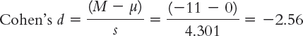
The effect size, d = −2.56, tells us that the sample mean difference and the population mean difference are 2.56 standard deviations apart. This is a large effect. Recall that the sign has no effect on the size of an effect: −2.56 and 2.56 are equivalent effect sizes. We can add the effect size when we report the statistics as follows: t(4) = −5.72, p < 0.05, d = −2.56.

CHECK YOUR LEARNING

Reviewing the Concepts

The paired-samples t test is used when we have data for all participants under two conditions—a within-groups design.
In the paired-samples t test, we calculate a difference score for every individual in the study. The statistic is calculated on those difference scores.
We use the same six steps of hypothesis testing that we used with the z test and with the single-sample t test.
We can calculate a confidence interval and an effect size for a paired-samples t test.

Clarifying the Concepts

9-10

How do we conduct a paired-samples t test?

9-11

Explain what an individual difference score is, as it is used in a paired-samples t test.

9-12

How does creating a confidence interval for a paired-samples t test give us the same information as hypothesis testing with a paired-samples t test?

9-13

How do we calculate Cohen’s d for a paired-samples t test?

Calculating the Statistics

9-14

Below are energy-level data (on a scale of 1 to 7, where 1 = feeling of no energy and 7 = feeling of high energy) for five students before and after lunch. Calculate the mean difference for these people so that loss of energy is a negative value. Assume you are testing the hypothesis that students go into what we call a “food coma” after eating, versus lunch giving them added energy.

Before Lunch	After Lunch
6	3
5	2
4	6
5	4
7	5

9-15

Assume that researchers asked five participants to rate their mood on a scale from 1 to 7 (1 being lowest, 7 being highest) before and after watching a funny video clip. The researchers reported that the average difference between the “before” mood score and the “after” mood score was M = 1.0, s = 1.225. They calculated a paired-samples t test, t(4) = 1.13, p > 0.05 and, using a two-tailed test with a p level of 0.05, failed to reject the null hypothesis.

Calculate the 95% confidence interval for this t test and describe how it results in the same conclusion as the hypothesis test.
Calculate and interpret Cohen’s d.

Applying the Concepts

9-16

Using the energy-level data presented in Check Your Learning 9-14, test the hypothesis that students have different energy levels before and after lunch. Perform the six steps of hypothesis testing for a two-tailed paired-samples t test.

9-17

Using the energy-level data, let’s go beyond hypothesis testing.

Calculate the 95% confidence interval and describe how it results in the same conclusion as the hypothesis test.
Calculate and interpret Cohen’s d.

Solutions to these Check Your Learning questions can be found in Appendix D.

235