9.2 The Single-Sample t Test
The single-
A single-
Specifically, a single-
The t Table and Degrees of Freedom
Degrees of freedom is the number of scores that are free to vary when we estimate a population parameter from a sample.
When we use the t distributions, we use the t table. There are different t distributions for every sample size and the t table takes sample size into account. However, we do not look up the actual sample size on the table. Rather, we look up degrees of freedom, the number of scores that are free to vary when we estimate a population parameter from a sample.
Language Alert! The phrase “free to vary” refers to the number of scores that can take on different values when a given parameter is known.
EXAMPLE 9.4
For example, the manager of a baseball team needs to assign nine players to particular spots in the batting order but only has to make eight decisions (N − 1). Why? Because only one option remains after making the first eight decisions. So before the manager makes any decisions, there are N − 1, or 9 − 1 = 8, degrees of freedom. After the second decision, there are N − 1, or 8 − 1 = 7, degrees of freedom, and so on.
MASTERING THE CONCEPT
9.2: Degrees of freedom refers to the number of scores that can take on different values when a given parameter is known. For example, if we know that the mean of three scores is 10, only two scores are free to vary. Once we know the values of two scores, we know the value of the third. If we know that two of the scores are 9 and 10, then we know that the third must be 11.
As in the baseball example, there is always one score that cannot vary once all of the others have been determined. For example, if we know that the mean of four scores is 6 and we know that three of the scores are 2, 4, and 8, then the last score must be 10. So the degrees of freedom is the number of scores in the sample minus 1. Degrees of freedom is written in symbolic notation as df, which is always italicized. The formula for degrees of freedom for a single-
MASTERING THE FORMULA
9-
df = N − 1
228
This is one key piece of information to keep in mind as we work with the t table. In the behavioral sciences, the degrees of freedom usually correspond to how many people are in the study or how many observations we make. If we were studying the number of followers of college students who use Twitter from a particular sample of college students to the average number of followers of all Twitter users, then the degrees of freedom would refer to how many college students were in the sample.
Table 9-1 is an excerpt from a t table; the full table is in Appendix B. Notice the relation between degrees of freedom and the critical value needed to declare statistical significance. In the column corresponding to a one-
| One- |
Two- |
|||||
|---|---|---|---|---|---|---|
| df | 0.10 | 0.05 | 0.01 | 0.10 | 0.05 | 0.01 |
| 1 | 3.078 | 6.314 | 31.821 | 6.314 | 12.706 | 63.657 |
| 2 | 1.886 | 2.920 | 6.965 | 2.920 | 4.303 | 9.925 |
| 3 | 1.638 | 2.353 | 4.541 | 2.353 | 3.182 | 5.841 |
| 4 | 1.533 | 2.132 | 3.747 | 2.132 | 2.776 | 4.604 |
| 5 | 1.476 | 2.015 | 3.365 | 2.015 | 2.571 | 4.032 |
The pattern continues when we have four observations (with df of 3). The critical t value needed to declare statistical significance decreases from 2.920 to 2.353. The level of confidence in the observations increases and the critical value decreases.
The t distributions become closer to the z distribution as sample size increases—
MASTERING THE CONCEPT
9.3: As sample size increases, the t distributions more and more closely approximate the z distribution. You can think of the z statistic as a single-
Check it out for yourself by comparing the z and t tables in Appendix B. For example, the z statistic for the 95th percentile—
229
Let’s remind ourselves why the t statistic merges with the z statistic as sample size increases. More participants in a study—
Let’s determine the cutoffs, or critical t value(s), for a research study using the full t table in Appendix B.
EXAMPLE 9.5
The study: A researcher knows the mean number of calories a rat will consume in half an hour if unlimited food is available. He wonders whether a new food will lead rats to consume a different number of calories—
The cutoff(s): This is a two-
df = N − 1 = 38 − 1 = 37
We want to look in the t table under two-
The Six Steps of the Single-Sample t Test
Now we have all the tools necessary to conduct a single-
EXAMPLE 9.6

Chapter 4 presented data that included the mean number of sessions attended by clients at a university counseling center. We noted that one study reported a mean of 4.6 sessions (Hatchett, 2003). Let’s imagine that the counseling center hoped to increase participation rates by having students sign a contract to attend at least 10 sessions. Five students sign the contract and attend 6, 6, 12, 7, and 8 sessions, respectively. The researchers are interested only in their university, so treat the mean of 4.6 sessions as a population mean.
STEP 1: Identify the populations, distribution, and assumptions.
Population 1: All clients at this counseling center who sign a contract to attend at least 10 sessions. Population 2: All clients at this counseling center who do not sign a contract to attend at least 10 sessions.
230
The comparison distribution will be a distribution of means. The hypothesis test will be a single-
This study meets one of the three assumptions and may meet the other two: (1) The dependent variable is scale. (2) We do not know whether the data were randomly selected, however, so we must be cautious with respect to generalizing to other clients at this university who might sign the contract. (3) We do not know whether the population is normally distributed, and there are not at least 30 participants. However, the data from the sample do not suggest a skewed distribution.
STEP 2: State the null and research hypotheses.
Null hypothesis: Clients at this university who sign a contract to attend at least 10 sessions attend the same number of sessions, on average, as clients who do not sign such a contract—
Research hypothesis: Clients at this university who sign a contract to attend at least 10 sessions attend a different number of sessions, on average, than do clients who do not sign such a contract—
STEP 3: Determine the characteristics of the comparison distribution.
μM = 4.6; sM = 1.114
Calculations:
| X | X − M | (X − M)2 |
|---|---|---|
| 6 | −1.8 | 3.24 |
| 6 | −1.8 | 3.24 |
| 12 | 4.2 | 17.64 |
| 7 | −0.8 | 0.64 |
| 8 | 0.2 | 0.04 |
The numerator of the standard deviation formula is the sum of squares:

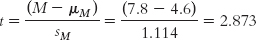
STEP 4: Determine the critical values, or cutoffs.
df = N − 1 = 5 − 1 = 4
For a two-
231
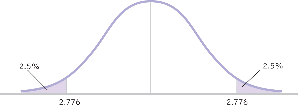
Figure 9-
STEP 5: Calculate the test statistic.
STEP 6: Make a decision.
Reject the null hypothesis. It appears that counseling center clients who sign a contract to attend at least 10 sessions do attend more sessions, on average, than do clients who do not sign such a contract (Figure 9-3).
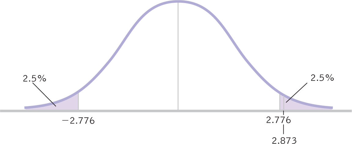
Figure 9-
After completing the hypothesis test, we want to present the primary statistical information in a report. There is a standard American Psychological Association (APA) format for the presentation of statistics across the behavioral sciences so that the results are easily understood by the reader.
- Write the symbol for the test statistic (e.g., t).
- Write the degrees of freedom, in parentheses.
- Write an equal sign and then the value of the test statistic, typically to two decimal places.
- Write a comma and then indicate the p value by writing “p = ” and then the actual value. (Unless we use software to conduct the hypothesis test, we will not know the actual p value associated with the test statistic. In this case, we simply state whether the p value is beyond the critical value by saying p < 0.05 when we reject the null hypothesis or p > 0.05 when we fail to reject the null hypothesis.)
In the counseling center example, the statistics would read:
t(4) = 2.87, p < 0.05
232
The statistics typically follow a statement about the finding; for example, “It appears that counseling center clients who sign a contract to attend at least 10 sessions do attend more sessions, on average, than do clients who do not sign such a contract, t(4) = 2.87, p < 0.05.” The report would also include the sample mean and standard deviation (not standard error) to two decimal points. Here, the descriptive statistics would read: (M = 7.80, SD = 2.49). By convention, we use SD instead of s to symbolize the standard deviation.
Calculating a Confidence Interval for a Single-Sample t Test
As it does with a z test, the APA recommends that researchers report confidence intervals and effect sizes, in addition to the results of hypothesis tests, whenever possible.
EXAMPLE 9.7
We can calculate a confidence interval with the single-
When we conducted hypothesis testing, we centered the curve around the mean according to the null hypothesis—
MASTERING THE CONCEPT
9.4: Whenever researchers conduct a hypothesis test, the APA encourages that, if possible, they also calculate a confidence interval and an effect size.
STEP 1: Draw a picture of a t distribution that includes the confidence interval.
We draw a normal curve (Figure 9-4) that has the sample mean, 7.8, at its center (instead of the population mean, 4.6).
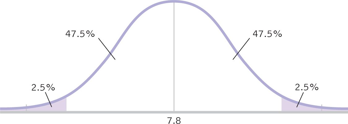
Figure 9-
STEP 2: Indicate the bounds of the confidence interval on the drawing.
We draw a vertical line from the mean to the top of the curve. For a 95% confidence interval, we also draw two much smaller vertical lines that indicate the middle 95% of the t distribution (2.5% in each tail, for a total of 5%). We then write the appropriate percentages under the segments of the curve.
STEP 3: Look up the t statistics that fall at each line marking the middle 95%.
For a two-
233
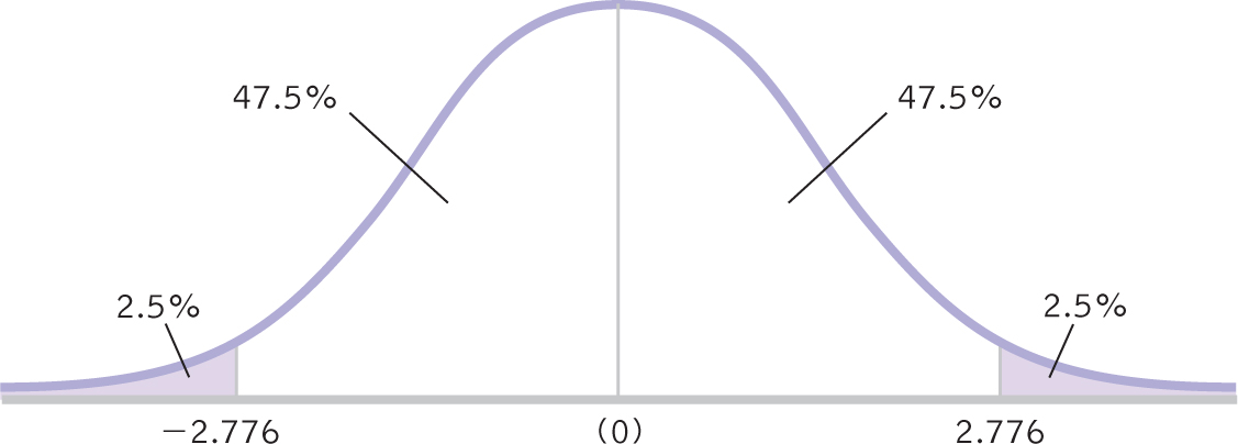
Figure 9-
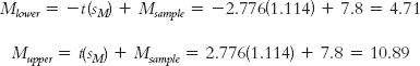
STEP 4: Convert the t statistics back into raw means.
As we did with the z test, we can use formulas for this conversion, but first we identify the appropriate mean and standard deviation. There are two important points to remember. First, we center the interval around the sample mean, so we use the sample mean of 7.8 in the calculations. Second, because we have a sample mean (rather than an individual score), we use a distribution of means. So we use the standard error of 1.114 as the measure of spread.
Using this mean and standard error, we calculate the raw mean at each end of the confidence interval, and add them to the curve, as in Figure 9-6. The formulas are exactly the same as for the z test except that z is replaced by t, and σM is replaced by sM.
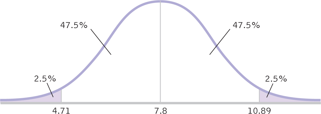
Figure 9-
MASTERING THE FORMULA
9-
The 95% confidence interval, reported in brackets as is typical, is [4.71, 10.89].
STEP 5: Verify that the confidence interval makes sense.
The sample mean should fall exactly in the middle of the two ends of the interval.
4.71 − 7.8 = −3.09; and 10.89 − 7.8 = 3.09
We have a match. The confidence interval ranges from 3.09 below the sample mean to 3.09 above the sample mean. If we were to sample five students from the same population over and over, the 95% confidence interval would include the population mean 95% of the time. Note that the population mean, 4.6, does not fall within this interval. This means it is not plausible that this sample of students who signed contracts came from the population according to the null hypothesis—
234
Calculating Effect Size for a Single-Sample t Test
As with a z test, we can calculate the effect size (Cohen’s d) for a single-
EXAMPLE 9.8
Let’s calculate the effect size for the counseling center study. Similar to what we did with the z test, we simply use the formula for the t statistic, substituting s for sM (and μ for μM, even though these means are always the same). This means we use 2.490 instead of 1.114 in the denominator. Cohen’s d is based on the spread of the distribution of individual scores, rather than the distribution of means.
MASTERING THE FORMULA
9- . It is the same formula as for the t statistic, except that we divide by the population standard deviation (s) rather than by the population standard error (sM).
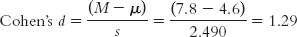
The effect size, d = 1.29, tells us that the sample mean and the population mean are 1.29 standard deviations apart. According to the conventions we learned in Chapter 8 (that 0.2 is a small effect, 0.5 is a medium effect, and 0.8 is a large effect), this is a large effect. We can add the effect size when we report the statistics as follows: t(4) = 2.87, p < 0.05, d = 1.29.
Next Steps
Dot Plots
When we conduct hypothesis tests such as the single-
MASTERING THE CONCEPT
9.5: A dot plot includes a dot for every score along an x-axis, listing the full range of possible values. It allows us to see the overall shape of a sample while also viewing every score. Dot plots also allow us to compare two samples because the dots for one sample are placed directly above the dots for the other.
The dot plot is a graph that displays all the data points in a sample, with the range of scores along the x-
The dot plot is a graph that displays all the data points in a sample, with the range of scores along the x-axis and a dot for each data point above the appropriate value. Dot plots serve a function similar to that of stem-
235
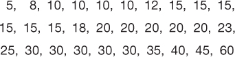
To demonstrate a dot plot, we’ll use the same data we used in Next Steps in Chapter 2—
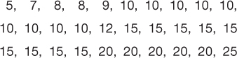
Here are the scores for 30 men in our statistics classes who also reported how many minutes they typically spend in the shower:
To create a dot plot, there are three basic steps.
STEP 1: Determine the lowest score and highest score of the sample.
These scores are 5 and 60 for women, and 5 and 25 for men.
STEP 2: Draw an x-axis and label it, including the values from the lowest through highest scores.
See Figure 9.7.
STEP 3: Place a dot above the appropriate value for every score.
See Figure 9.7.
Figure 9-7 displays a stacked dot plot for the samples of male and female students’ minutes spent in the shower. With the dot plot, we can easily observe the slightly higher central tendency and larger spread for the women than the men, as well as the potential outlier in the female sample.
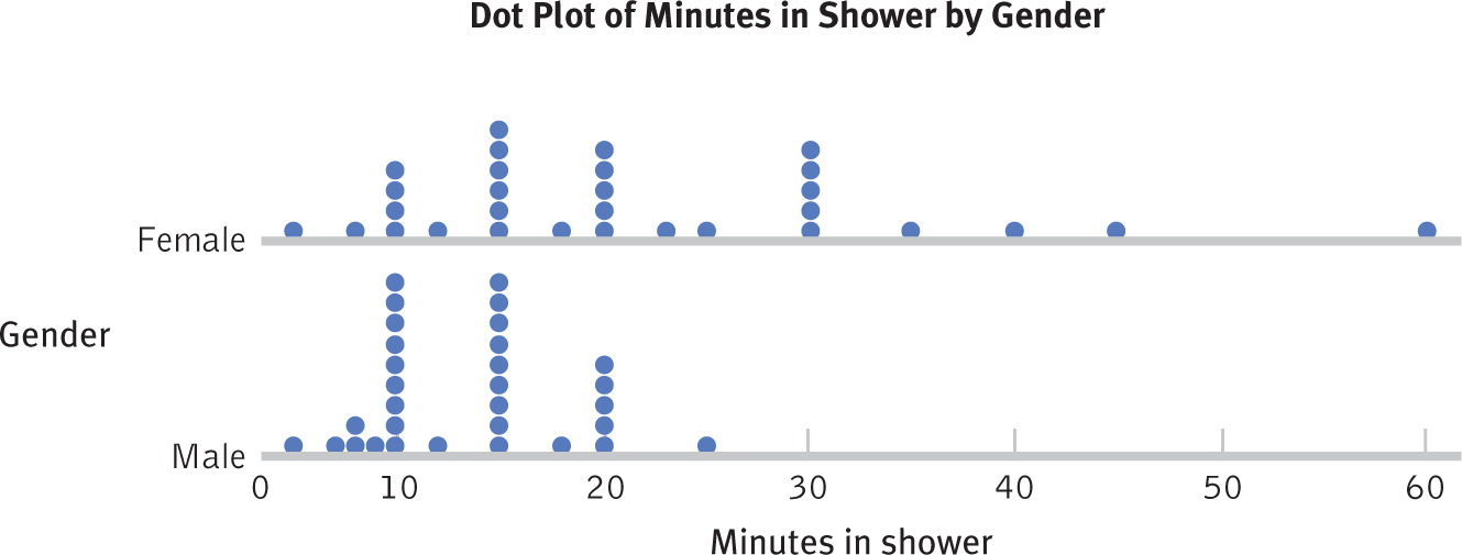
Figure 9-
236
CHECK YOUR LEARNING
Reviewing the Concepts
- A single-
sample t test is used to compare data from one sample to a population for which we know the mean but not the standard deviation. - We consider degrees of freedom, or the number of scores that are free to vary, instead of N when we assess estimated test statistics against distributions.
- As sample size increases, confidence in the estimates improves, degrees of freedom increase, and the critical value, for t drop, making it easier to reach statistical significance. In fact, as sample size grows, the t distributions approach the z distribution.
- To conduct a single-
sample t test, we follow the same six steps of hypothesis testing as the z test, except that we estimate the standard deviation from the sample before we calculate standard error. - We can calculate a confidence interval and an effect size, Cohen’s d, for a single-
sample t test. - Dot plots allow us to view the shape of a sample’s distribution as well as every single data point in that sample. They also depict the scores of two samples on top of one another to allow for easy comparisons of distributions.
Clarifying the Concepts
- 9-
5 Explain the term degrees of freedom. - 9-
6 Why is a single-sample t test more useful than a z test?
Calculating the Statistics
- 9-
7 Compute degrees of freedom for each of the following:- An experimenter times how long it takes 35 rats to run through a maze with eight pathways.
- Test scores for 14 students are collected and averaged over four semesters.
- 9-
8 Identify the critical t value for each of the following tests:- A two-
tailed test with alpha of 0.05 and 11 degrees of freedom - A one-
tailed test with alpha of 0.01 and N of 17
- A two-
Applying the Concepts
- 9-
9 Let’s assume that according to university summary statistics, the average student misses 3.7 classes during a semester. Imagine the data you have been working with (6, 3, 7, 6, 4, 5) for the number of classes missed by a group of students. Conduct all six steps of hypothesis testing, using a two-tailed test with a p level of 0.05. (Note: You completed the work for step 3 in Check Your Learning 9- 2 and 9- 3.)
Solutions to these Check Your Learning questions can be found in Appendix D.