7.3 Additional Topics on Inference
 This page includes Statistical Videos
In this section, we discuss two topics that are related to the procedures we have learned for inference about population means. First, we focus on an important issue when planning a study, specifically choosing the sample size. A wise user of statistics does not plan for inference without at the same time planning data collection. The second topic introduces us to various inference methods for non-Normal populations. These would be used when our populations are clearly non-Normal and we do not think that the sample size is large enough to rely on the robustness of the t procedures.
Choosing the sample size
We describe sample size procedures for both confidence intervals and significance tests. For anyone planning to design a study, a general understanding of these procedures is necessary. While the actual formulas are a bit technical, statistical software now makes it trivial to get sample size results.
Sample size for confidence intervals
We can arrange to have both high confidence and a small margin of error by choosing an appropriate sample size. Let’s first focus on the one sample t confidence interval. Its margin of error is
m=t*SEˉx=t*s√n
Besides the confidence level C and sample size n, this margin of error depends on the sample standard deviation s. Because we don’t know the value of s until we collect the data, we guess a value to use in the calculations. Thus, because s is our estimate of the population standard deviation σ this value can also be considered our guess of the population standard deviation.

We will call this guessed value s*. We typically guess at this value using results from a pilot study or from similar studies published earlier. It is always better to use a value of the standard deviation that is a little larger than what is expected. This may result in a sample size that is a little larger than needed, but it helps avoid the situation where the resulting margin of error is larger than desired.
Given an estimate for s and the desired margin of error m, we can find the sample size by plugging everything into the margin of error formula and solving for n. The one complication, however, is that t* depends not only on the confidence level C but also on the sample size n. Here are the details.
Sample Size for Desired Margin of Error for a Mean μ
The level C confidence interval for a mean μ will have an expected margin of error less than or equal to a specified value m when the sample size is such that
m≥t*s*/√n
Here t* is the critical value for confidence level C with n−1 degrees of freedom, and s* is the guessed value for the population standard deviation.
Finding the smallest sample size n that satisfies this requirement can be done using the following iterative search:
- Get an initial sample size by replacing t* with z*. Compute n=(z*s*/m)2 and round up to the nearest integer.
- Use this sample size to obtain t*, and check if m≥t*s*/√n.
- If the requirement is satisfied, then this n is the needed sample size. If the requirement is not satisfied, increase n by 1 and return to Step 2.
Notice that this method makes no reference to the size of the population. It is the size of the sample that determines the margin of error. The size of the population does not influence the sample size we need as long as the population is much larger than the sample. Here is an example.
EXAMPLE 7.16 Planning a Survey of College Students
In Example 7.1 (page 361), we calculated a 95% confidence interval for the mean minutes per day a college student at your institution uses a smartphone. The margin of error based on an SRS of n=8 students was 21.2 minutes. Suppose that a new study is being planned and the goal is to have a margin of error of 15 minutes. How many students need to be sampled?
The sample standard deviation in Example 7.1 was 25.33. To be conservative, we’ll guess that the population standard deviation is 30 minutes.
To compute an initial n, we replace t* with z*. This results in
n=(z*s*m)2=[1.96(30)15]2=15.37
Round up to get n=16.
We now check to see if this sample size satisfies the requirement when we switch back to t*. For n=16, we have n−1=15 degrees of freedom and t*=2.131. Using this value, the expected margin of error is
2.131(30.00)/√16=15.98
This is larger than m=15, so the requirement is not satisfied.
The following table summarizes these calculations for some larger values of C.
n t*s*/√n 16 15.98 17 15.43 18 14.92 19 14.46
The requirement is first satisfied when n=18. Thus, we need to sample at least n=18 students for the expected margin of error to be no more than 15 minutes.
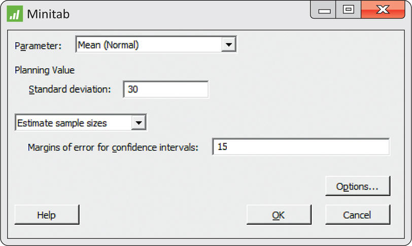
Figure 7.12 shows the Minitab input window needed to do these calculations Because the default confidence level is 95%, only the desired margin of error m and the estimate for s need to be entered.
Note that the n=18 refers to the expected margin of error being no more than 15 minutes. This does not guarantee that the margin of error for the sample we collect will be less than 15 minutes. That is because the sample standard deviation s varies sample to sample and these calculations are treating it as a fixed quantity. More advanced sample size procedures ask you to also specify the probability of obtaining a margin of error less than the desired value. For our approach, this probability is roughly 50%. For a probability closer to 100%, the sample size will need to be larger. For example, suppose we wanted this probability to be roughly 80%. In SAS, we’d perform these calculations using the command
proc power;
onesamplemeans CI=t stddev=30 halfwidth=15
probwidth=0.80 ntotal=.;
run;
The needed sample size increases from n=18 to n=22.
Unfortunately, the actual number of usable observations is often less than that planned at the beginning of a study. This is particularly true of data collected in surveys or studies that involve a time commitment from the participants. Careful study designers often assume a nonresponse rate or dropout rate that specifies what proportion of the originally planned sample will fail to provide data. We use this information to calculate the sample size to be used at the start of the study. For example, if in the preceding survey we expect only 25% of those students to respond, we would need to start with a sample size of 4×18=72 to obtain usable information from 18 students.
These sample size calculations also do not account for collection costs. In practice, taking observations costs time and money. There are times when the required sample size may be impossibly expensive. In those situations, one might consider a larger margin of error and/or a lower confidence level to be acceptable.
For the two-sample t confidence interval, the margin of error is
m=t*√s21n1+s22n2
A similar type of iterative search can be used to determine the sample sizes n1 and n2, but now we need to guess both standard deviations and decide on an estimate for the degrees of freedom. We suggest taking the conservative approach and using the smaller of n1−1 and n2−1 for the degrees of freedom. Another approach is to consider the standard deviations and sample sizes are equal, so the margin of error is
m=t*√2s2n
and use degrees of freedom 2(n−1). That is the approach most statistical software take.
EXAMPLE 7.17 Planning a New Smart Shopping Cart Study
smrtcrt
As part of Example 7.10 (pages 381–382), we calculated a 95% confidence interval for the mean difference in spending when shopping with and without real-time feedback. The 95% margin of error was roughly $2.70. Suppose that a new study is being planned and the desired margin of error is $1.50. How many shoppers per group do we need?
The sample standard deviations in Example 7.10 were $6.59 and $6.85. To be a bit conservative, we’ll guess that the two population standard deviations are both $7.00. To compute an initial n, we replace t* with z*. This results in
n=(√2z*s*m)2=[√2(1.96)(7)1.5]2=167.3
We round up to get n=168. The following table summarizes the margin of error for this and some larger values of n.
| n | t*s*√2/n |
|---|---|
| 168 | 1.502 |
| 169 | 1.498 |
| 170 | 1.493 |
The requirement is first satisfied when n=169. In SAS, we’d perform these calculations using the command
proc power;
twosamplemeans CI=diff stddev=7 halfwidth=1.5
probwidth=0.50 npergroup=.;
run;
This sample size is almost 3.5 times the sample size used in Example 7.10. The researcher may not be able to recruit this large a sample. If so, we should consider a larger desired margin of error.
Apply Your Knowledge
Question 7.75
7.75 Starting salaries
In a recent survey by the National Association of Colleges and Employers, the average starting salary for computer science majors was reported to be $61,741.32 You are planning to do a survey of starting salaries for recent computer science majors from your university. Using an estimated standard deviation of $15,300, what sample size do you need to have a margin of error equal to $5000 with 95% confidence?
7.75
n=40. Answers may vary if using software.
Question 7.76
7.76 Changes in sample size
Suppose that, in the setting of the previous exercise, you have the resources to contact 40 recent graduates. If all respond, will your margin of error be larger or smaller than $5000? What if only 50% respond? Verify your answers by performing the calculations.
The power of the one-sample t test
The power of a statistical test measures its ability to detect deviations from the null hypothesis. Because we usually hope to show that the null hypothesis is false, it is important to design a study with high power. Power calculations are a way to assess whether or not a sample size is sufficiently large to answer the research question.
The power of the one-sample t test against a specific alternative value of the population mean μ is the probability that the test will reject the null hypothesis when this alternative is true. To calculate the power, we assume a fixed level of significance, usually α=0.05.
Calculation of the exact power of the t test takes into account the estimation of σ by s and requires a new distribution. We will describe that calculation when discussing the power of the two-sample t test. Fortunately, an approximate calculation that is based on assuming that σ is known is generally adequate for planning most studies in the one-sample case. This calculation is very much like that for the z test, presented in Section 6.5. The steps are

- Write the event, in terms of ˉx, that the test rejects H0.
- Find the probability of this event when the population mean has the alternative value.
Here is an example.
EXAMPLE 7.18 Is the Sample Size Large Enough?
Recall Example 7.2 (pages 363–364) on the daily amount of time using a smartphone. A friend of yours is planning to compare her institutional average with the UK average of 119 minutes per day. She decides that a mean at least 10 minutes smaller is useful in practice. Can she rely on a sample of 10 students to detect a difference of this size?
She wishes to compute the power of the t test for
H0:μ=119Ha:μ<119
against the alternative that μ=119−10=109 when n=10. This gives us most of the information we need to compute the power. The other important piece is a rough guess of the size of σ. In planning a large study, a pilot study is often run for this and other purposes. In this case, she can use the standard deviation from your institution. She will therefore round up and use σ=30 and s=30 in the approximate calculation.
Step 1. The t test with 10 observations rejects H0 at the 5% significance level if the t statistic
t=ˉx−119s/√10
is less than the lower 5% point of t(9), which is −1.833. Taking s=30, the event that the test rejects H0 is, therefore,
t=ˉx−11930/√10≤−1.833ˉx≤119−1.83330√10ˉx≤101.61
Step 2. The power is the probability that ˉx≤101.61 when μ=109. Taking σ=30, we find this probability by standardizing ˉx:
P(ˉx≤101.61 when μ=109)=P(ˉx−10930/√10≤101.61−10930/√10)=P(Z≤−0.7790)=0.2177
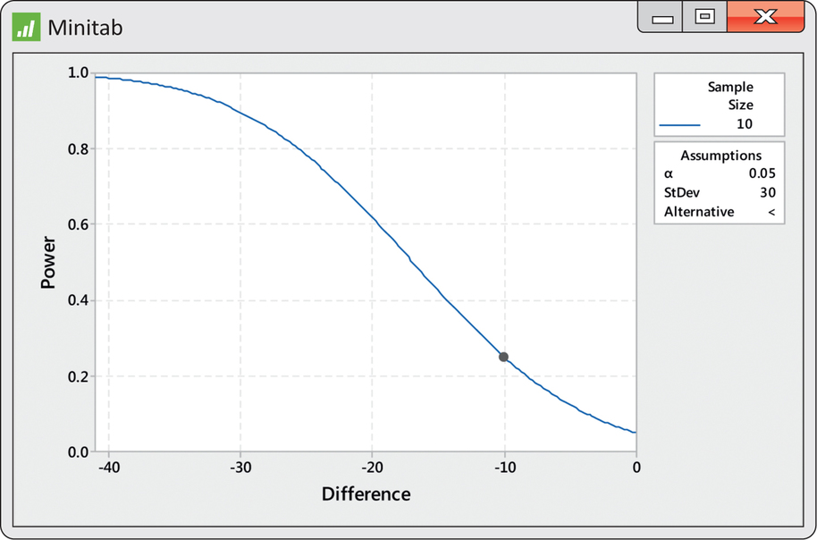
A mean value of 109 minutes will produce significance at the 5% level in only 21.8% of all possible samples. Figure 7.13 shows Minitab output for the exact power calculation. It is about 25% and is represented by a dot on the power curve at a difference of −10. This curve is very informative. We see that with a sample size of 10, the power is greater than 80% only for differences larger than about 26 minutes. Your friend will definitely want to increase the sample size.
Apply Your Knowledge
Question 7.77
7.77 Power for other values of μ.
If you repeat the calculation in Example 7.18 for values of μ that are smaller than 109, would you expect the power to be higher or lower than 0.2177? Why?
7.77
Higher, if the alternative μ is farther away from 119 then we will have more power.
Question 7.78
7.78 Another power calculation
Verify your answer to the previous exercise by doing the calculation for the alternative μ=99 minutes.
The power of the two-sample t test
The two-sample t test is one of the most used statistical procedures. Unfortunately, because of inadequate planning, users frequently fail to find evidence for the effects that they believe to be present. This is often the result of an inadequate sample size. Power calculations, performed prior to running the experiment, will help avoid this occurrence.
We just learned how to approximate the power of the one-sample t test. The basic idea is the same for the two-sample case, but we will describe the exact method rather than an approximation again. The exact power calculation involves a new distribution, the noncentral t distribution. This calculation is not practical by hand but is easy with software that calculates probabilities for this new distribution.
noncentral t distribution
We consider only the common case where the null hypothesis is “no difference,” μ1−μ2=0. We illustrate the calculation for the pooled two-sample t test. A simple modification is needed when we do not pool. The unknown parameters in the pooled t setting are μ1,μ2, and a single common standard deviation σ. To find the power for the pooled two-sample t test, follow these steps.
Step 1. Specify these quantities:
- an alternative value for μ1−μ2 that you consider important to detect;
- the sample sizes, n1 and n2;
- a fixed significance level α, often α=0.05; and
- an estimate of the standard deviation σ from a pilot study or previous studies under similar conditions.
Step 2. Find the degrees of freedom df=n1+n2−2 and the value of t* that will lead to rejecting H0 at your chosen level α.
noncentrality parameter
Step 3. Calculate the noncentrality parameter
δ=|μ1−μ2|σ√1n1+1n2
Step 4. The power is the probability that a noncentral t random variable with degrees of freedom df and noncentrality parameter δ will be greater than t∗. Use software to calculate this probability. In SAS, the command is 1-PROBT(tstar, df,delta). If you do not have software that can perform this calculation, you can approximate the power as the probability that a standard Normal random variable is greater than t∗−δ, that is, P(Z>t∗−δ). Use Table A or software for standard Normal probabilities.
Note that the denominator in the noncentrality parameter,
σ√1n1+1n2
is our guess at the standard error for the difference in the sample means. Therefore, if we wanted to assess a possible study in terms of the margin of error for the estimated difference, we would examine t∗ times this quantity.
If we do not assume that the standard deviations are equal, we need to guess both standard deviations and then combine these to get an estimate of the standard error:
√σ21n1+σ22n2
This guess is then used in the denominator of the noncentrality parameter. Use the conservative value, the smaller of n1−1 and n2−1, for the degrees of freedom.
EXAMPLE 7.19 Active versus Failed Companies
CASE 7.2 In Case 7.2, we compared the cash flow margin for 74 active and 27 failed companies. Using the pooled two-sample procedure, the difference was statistically significant (t=2.82,df=99,P=0.005). Because this study is a year old, let’s plan a similar study to determine if these findings continue to hold.
Should our new sample have similar numbers of firms? Or could we save resources by using smaller samples and still be able to declare that the successful and failed firms are different? To answer this question, we do a power calculation.
Step 1. We want to be able to detect a difference in the means that is about the same as the value that we observed in our previous study. So, in our calculations, we will use μ1−μ2=12.00. We are willing to assume that the standard deviations will be about the same as in the earlier study, so we take the standard deviation for each of the two groups of firms to be the pooled value from our previous study, σ=19.59.
We need only two pieces of additional information: a significance level α and the sample sizes n1 and n2. For the first, we will choose the standard value α=0.05. For the sample sizes, we want to try several different values. Let’s start with n1=26 and n2=26.
Step 2. The degrees of freedom are n1+n2−2=50. The critical value is t∗=2.009, the value from Table D for a two-sided α=0.05 significance test based on 50 degrees of freedom.
Step 3. The noncentrality parameter is
δ=12.0019.59√126+126=12.005.43=2.21
Step 4. Software gives the power as 0.582. The Normal approximation is very accurate:
P(Z>t∗−δ)=P(Z>−0.201)=0.5793
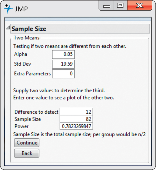
If we repeat the calculation with n1=41 and n2=41, we get a power of 78%. This result using JMP is shown in Figure 7.14. We need a relatively large sample to detect this difference.
Apply Your Knowledge
Question 7.79
7.79 Power and μ1−μ2
If you repeat the calculation in Example 7.19 for other values of μ1−μ2 that are smaller than 12, would you expect the power to increase or decrease? Explain.
7.79
Decrease, because the difference we are trying to find is smaller, it is harder to detect, so the power will be smaller.
Question 7.80
7.80 Power and the standard deviation
If the true population standard deviation were 25 instead of the 19.59 hypothesized in Example 7.19, would the power increase or decrease? Explain.
Inference for non-Normal populations
We have not discussed how to do inference about the mean of a clearly non-Normal distribution based on a small sample. If you face this problem, you should consult an expert. Three general strategies are available:
- In some cases, a distribution other than a Normal distribution describes the data well. There are many non-Normal models for data, and inference procedures for these models are available.
- Because skewness is the chief barrier to the use of t procedures on data without outliers, you can attempt to transform skewed data so that the distribution is symmetric and as close to Normal as possible. Confidence levels and P-values from the t procedures applied to the transformed data will be quite accurate for even moderate sample sizes. Methods are generally available for transforming the results back to the original scale.
- The third strategy is to use a distribution-free inference procedure. Such procedures do not assume that the population distribution has any specific form, such as Normal. Distribution-free procedures are often called nonparametric procedures. The bootstrap is a modern computer-intensive nonparametric procedure that is especially useful for confidence intervals. Chapter 16 discusses traditional nonparametric procedures, especially significance tests.
distribution-free procedures
nonparametric procedures
Each of these strategies quickly carries us beyond the basic practice of statistics. We emphasize procedures based on Normal distributions because they are the most common in practice, because their robustness makes them widely useful, and (most importantly) because we are first of all concerned with understanding the principles of inference.
Distribution-free significance tests do not require that the data follow any specific type of distribution such as Normal. This gain in generality isn’t free: if the data really are close to Normal, distribution-free tests have less power than t tests. They also don’t quite answer the same question. The t tests concern the population mean. Distribution-free tests ask about the population median, as is natural for distributions that may be skewed.
The sign test
sign test
The simplest distribution-free test, and one of the most useful, is the sign test. The test gets its name from the fact that we look only at the signs of the differences, not their actual values. The following example illustrates this test.
EXAMPLE 7.20 The Effects of Altering a Software Parameter
geparts
Example 7.7 (pages 368–370) describes an experiment to compare the measurements obtained from two software algorithms. In that example we used the matched pairs t test on these data, despite some skewness, which make the P-value only roughly correct. The sign test is based on the following simple observation: of the 76 parts measured, 43 had a larger measurement with the option off and 33 had a larger measurement with the option on.
To perform a significance test based on these counts, let p be the probability that a randomly chosen part would have a larger measurement with the option turned on. The null hypothesis of “no effect” says that these two measurements are just repeat measurements, so the measurement with the option on is equally likely to be larger or smaller than the measurement with the option off. Therefore, we want to test
H0:p=1/2Ha:p≠1/2
The 76 parts are independent trials, so the number that had larger measurements with the option off has the binomial distribution B(76,1/2) if H0 is true. The P-value for the observed count 43 is, therefore, 2P(X≥43), where X has the B(76,1/2) distribution. You can compute this probability with software or the Normal approximation to the binomial:
2P(X≥43)=2P(Z≥43−38√19)=2P(Z≥1.147)=2(0.1251)=0.2502
As in Example 7.7, there is not strong evidence that the two measurements are different.
There are several varieties of the sign test, all based on counts and the binomial distribution. The sign test for matched pairs is the most useful. The null hypothesis of “no effect” is then always H0:p=1/2. The alternative can be one-sided in either direction or two-sided, depending on the type of change we are considering.
Sign Test for Matched Pairs
Ignore pairs with difference 0; the number of trials n is the count of the remaining pairs. The test statistic is the count X of pairs with a positive difference. P-values for X are based on the binomial B(n,1/2) distribution.
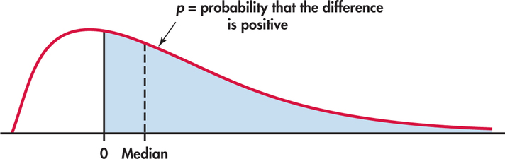
The matched pairs t test in Example 7.7 tested the hypothesis that the mean of the distribution of differences is 0. The sign test in Example 7.20 is, in fact, testing the hypothesis that the median of the differences is 0. If p is the probability that a difference is positive, then p=1/2 when the median is 0. This is true because the median of the distribution is the point with probability 1/2 lying to its right. As Figure 7.15 illustrates, p>1/2 when the median is greater than 0, again because the probability to the right of the median is always 1/2. The sign test of H0:p=1/2 against Ha:p>1/2 is a test of
H0:population median=0Ha:population median>0
The sign test in Example 7.20 makes no use of the actual scores—it just counts how many parts had a larger measurement with the option off. Any parts that did not have different measurements would be ignored altogether. Because the sign test uses so little of the available information, it is much less powerful than the t test when the population is close to Normal. Chapter 16 describes other distribution-free tests that are more powerful than the sign test.
Apply Your Knowledge
Question 7.81
7.81 Sign test for the oil-free frying comparison
Exercise 7.10 (page 371) gives data on the taste of hash browns made using a hot-oil fryer and an oil-free fryer. Is there evidence that the medians are different? State the hypotheses, carry out the sign test, and report your conclusion.
7.81
H0:p=0.5, Ha:p=0.5.
Using B(5, 0.5), 2P(X≥4)=2(0.1875)=0.375. There is no strong evidence that the two measurements are different.