Parasites have evolved offensive strategies while hosts have evolved defensive strategies
Parasites gain fitness when they find a suitable host and reproduce. Hosts will experience higher fitness if they avoid being parasitized. Therefore, natural selection has favored the evolution of parasite offenses and host defenses. In this section, we will examine some of these strategies as well as look at evolutionary relationships between parasites and hosts.
Parasite Adaptations
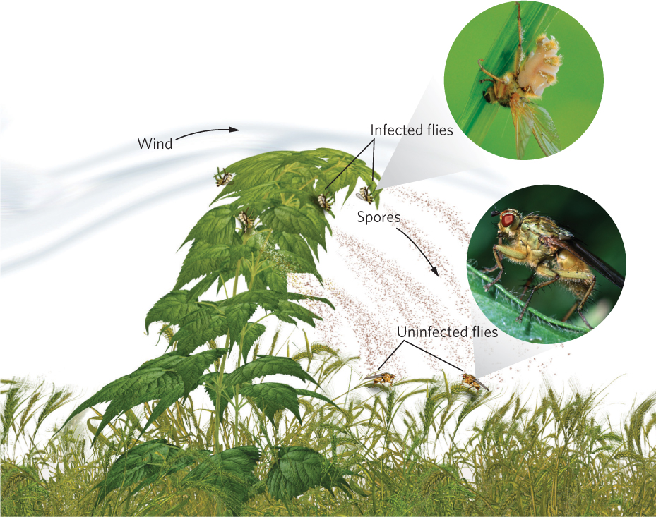
As we saw at the beginning of the chapter, parasites have evolved a wide array of strategies for finding and infecting hosts. Some of the most fascinating examples of parasite adaptation involve strategies that increase the probability of parasite transmission. For example, the pathogenic fungus Entomorpha muscae infects both houseflies (Musca domestica) and yellow dungflies (Scatophaga stercoraria). To improve its chance of transmitting its spores, it has two different strategies. When the fungus infects and kills female houseflies, the bodies become attractive to male houseflies looking for a mate. Although it is unclear what attractive cues the fungus produces, when a male housefly tries to mate with a dead female, spores of the fungus are transferred to the male’s body.
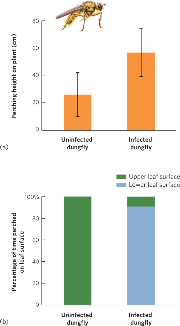
When the same fungus infects the yellow dungfly, the fly climbs up nearby vegetation, moves to the upwind side of the plant, and hangs upside down on the underside of a leaf. The fly then moves its wings toward the leaf, and moves its abdomen—which is swollen with fungal spores—away from the leaf. Once it reaches this position, the dungfly dies and the fungal spores erupt from its abdomen. The erupting spores can then potentially infect dungflies that pass below, as illustrated in Figure 15.16. When researchers compared the behavior of infected dungflies to uninfected dungflies, they found that uninfected flies perched lower on plants and never perched on the underside. You can view these data in Figure 15.17.
For parasites that require a series of different hosts to complete their life stages, it is challenging to find a way to get transmitted from one host to another. Some parasites—such as trematodes that first infect snails and subsequently infect tadpoles—have evolved a simple strategy of leaving the body of the first host and then searching for the second host. Other parasites have evolved ways of manipulating the behavior of the first host to ensure that the second host consumes it. We saw an example of this with the amber snail discussed at the beginning of the chapter. There are many examples of parasites taking control of the host’s behavior. For example, mice can inadvertently consume a parasitic protist, Toxoplasma gondii, when feeding near cat feces. Once the mouse becomes infected, it no longer avoids an area marked by the smell of bobcat (Lynx rufus) urine but, instead, is mildly attracted to it. As a result, the mouse is more likely to be eaten by the bobcat, which is a valuable outcome for the protist since it can only reproduce in the gut of a cat.
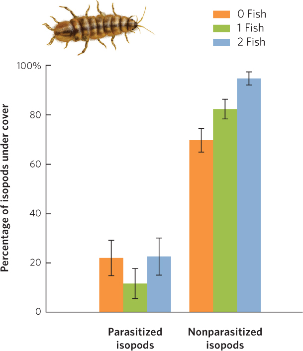
Similarly, small crustaceans known as isopods (Caecidotea intermedius) normally hide in refuges from predatory fish. However, if the isopods are infected by a parasitic worm (Acanthocephalus dirus), they spend less time in the refuge and more time out in the open where the fish are more likely to notice them, as you can see in Figure 15.18. This manipulation of the isopod’s behavior is beneficial to the parasite because fish serve as the parasite’s second host.
359
Host Adaptations
Host species have evolved a range of defenses to combat parasite invaders. Earlier in the chapter we noted that the immune system detects parasites that attempt to enter the body and tries to kill them. Other elements of the immune system are more general and do not recognize particular species of pathogens as foreign organisms. Some species of plants and animals can produce antibacterial and antifungal chemicals that kill bacterial and fungal parasites. For example, researchers have recently reported that many species of amphibians naturally release antimicrobial peptides onto their skin, which inhibit the growth of the deadly chytrid fungus.
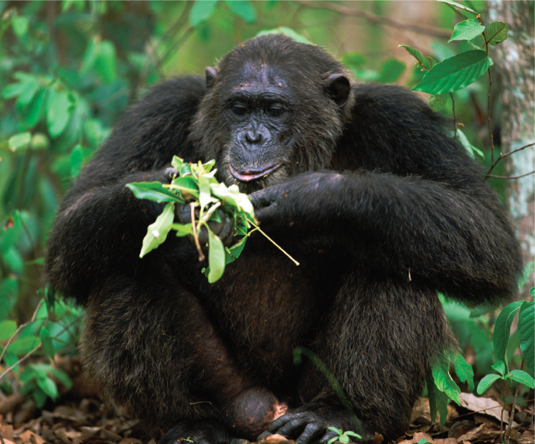
Host species have also evolved mechanical and biochemical defenses to combat parasites. We see this with chimpanzees living in Tanzania that become infected with intestinal worms. Instead of eating their normal food diet, chimps that are ill with the intestinal worms pick a few leaves from plants in the genus Aspilia and swallow them whole (Figure 15.19). The leaves of these plants are covered in tiny hooks and, as the leaves pass through the chimp’s digestive system, the hooks pull nematode parasites (Oesophagostomum stephanostomum) out of the digestive tract so they can be expelled from the chimp’s body with feces. Infected chimps also chew on bitter twigs from the Vernonia plant, something that healthy chimps do not do. The sick chimps become well within 24 hours because the twigs contain chemicals that kill a variety of different parasites. These plants are also consumed by people in the region when they experience symptoms of parasite infections. In short, both chimps and humans use plants to medicate themselves against parasitic infections.
360
Coevolution
When we consider the evolutionary forces that affect adaptations of parasites and hosts, we often find that as one species in the interaction adapts, the other species responds by adapting as well. As we discussed in Chapter 14, when two or more species continue to evolve in response to each other’s evolution we call it coevolution. When all species involved in an interaction coevolve together, no one species is likely to get an upper hand. For example, when a parasite evolves an advantage that makes it more effective at infecting hosts, the hosts will then be under stronger selection to evolve defenses against that parasite.
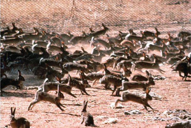
We can see an example of coevolution between parasites and hosts in the case of rabbits in Australia. In the 1800s European rabbits were introduced to many regions of the world where they had not lived historically. In Australia, for instance, rabbits were first introduced from England in 1859. Within a few years, local ranchers were erecting fences to keep them out and organizing shooting parties to help control the size of the population. Eventually, hundreds of millions of rabbits ranged throughout most of the continent, destroying sheep pasturelands and thereby threatening wool production (Figure 15.20). The Australian government tried poisons, predators, and other control measures, all without success.
ANALYZING ECOLOGY
Comparing Two Groups with a t-Test
When the dungfly researchers examined the perching height of infected and uninfected flies, they concluded that the infected flies perched significantly higher on vegetation. How did they come to that conclusion? They compared the mean heights for the infected and uninfected flies and used a statistical test to determine if the two means were different.
In Chapter 14, we discussed how scientists typically consider two means to be different if we can sample their distributions many times and find that the means of those sampled distributions overlap less than 5 percent of the time. We commonly call this critical cutoff alpha— abbreviated as α. Therefore we say that our critical cutoff is α = 0.05. To determine if the means of the two groups are significantly different, we need to know three things from each group: the mean, the variance, and the sample size.
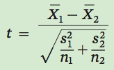
With these three parameters, we can calculate a t-test, which is a test that determines if the distributions of data from two groups are significantly different. An important assumption of the t-test is that the values from both groups are normally distributed.
We begin by calculating the differences between the means of the two groups:

where  is the mean of group 1 and
  is the mean of group 2.
Next we calculate the standard error of the difference in the two means:
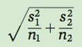
where  is the sample variance of group 1,
  is the sample variance of group 2, n1 is the sample size of group 1, and n2 is the sample size of group 2 (you can review the concept of sample variances in Chapter 2).
The next step is to divide the first calculated value by the second calculated value:
361
As you can see from this equation, the value of t becomes larger as the difference between the means becomes larger, or the standard error of the difference in the means becomes smaller.
For example, consider two groups of data with the following parameters:

In this case:
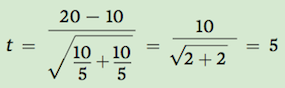
The last thing we need to calculate is known as the degrees of freedom, which is defined as the sum of the two sample sizes minus 2. In this example, the degrees of freedom is:
5 + 5 − 2 = 8
With this value of t calculated, we can then determine if our value exceeds a critical level of t and therefore determine whether the means are significantly different. We can find the critical value of t from a statistical table. If you look at the t-table in the “Statistical Tables” section at the back of this book, you can find the column that uses an alpha value of 0.05 and then find the row that contains 8 degrees of freedom. The critical t-value is the number found in this row and column. In this case, the critical t-value is 2.3. Because our calculated t-value exceeds the critical t-value, we can conclude that the two means differ significantly.
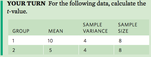
Next calculate the degrees of freedom.
Based on your calculated t-value and the critical t-value using α = 0.05, determine if the two groups are significantly different.

In 1950 the government tried a new approach. A virus known as Myxoma had been discovered in South American rabbits. The virus—which was carried by mosquitoes—causes a disease known as myxomatosis. The disease had minor effects on South American rabbits, but it turned out to be highly lethal to European rabbits; an infected rabbit dies within 48 hours. The Australian government introduced the virus and initially it had a devastating effect on the rabbits. Among infected rabbits, 99.8 percent died and the rabbit population declined to very low numbers. However, 0.2 percent of the infected rabbits proved to be resistant and passed on their resistant genes. Before the introduction of the Myxoma virus, a few rabbits possessed resistant genes, but they had never been favored. In a second outbreak of the disease, only 90 percent of infected rabbits died. By the third outbreak, only 40 to 60 percent of the rabbits died and the rabbit population of Australia started to increase. You can see the decline in rabbit mortality over time in Figure 15.21.
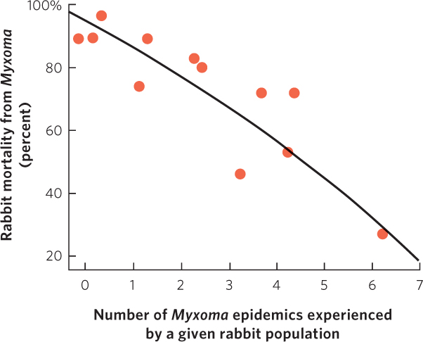
The declining percentage of rabbits that died was due partly to the evolution of increased resistance in the rabbit population, but because the rabbit population was initially killed in large numbers, the rapidly dwindling host population also favored any virus strains that infected the rabbits without killing them. Dead rabbits represent a dead end for the virus, especially if the rabbit dies before it is bitten by a mosquito, which is the only way the virus can be transmitted.
362
Over time, the interaction between the rabbits and the Myxoma virus resulted in a more resistant host population and a less lethal pathogen. This allowed the rabbit population to rebound and the virus to persist. This dynamic is probably what researchers observed in South America, where the rabbit population and Myxoma virus persisted together for a long time. To meet the Australian government’s goal of controlling the rabbit population in Australia, scientists continue to introduce new strains of the virus that are highly lethal to rabbits because the new strains have no history of coevolution with the Australian rabbits. In this way, they maintain the effectiveness of the Myxoma virus as a pest control agent.
ECOLOGY TODAY CONNECTING THE CONCEPTS
OF MICE AND MEN … AND LYME DISEASE
Back in the 1970s, a number of children in a Connecticut community experienced a suite of mysterious symptoms. Many had a bull’s-eye–shaped rash on their skin followed by flulike symptoms that developed into other symptoms similar to arthritis and various neurological disorders. Physicians discovered that the children had been infected by a pathogenic bacterium (Borrelia burgdorferi). Because the community was in the town of Lyme, Connecticut, the disease came to be known as Lyme disease.
363
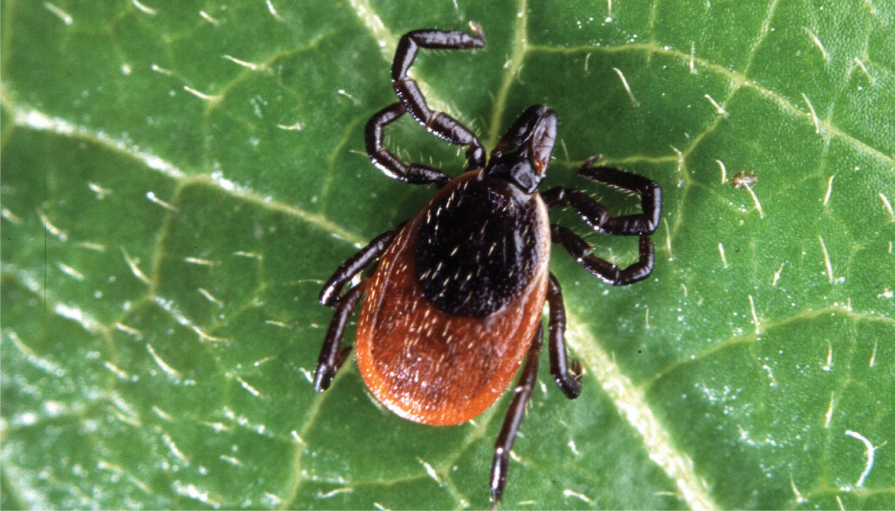
The parasite that causes Lyme disease is carried by ticks that feed on wild animals. Occasionally these ticks latch onto people and transmit the parasite. In North America, the primary vector is the black-legged tick (Ixodes scapularis), also known as the deer tick. The ticks and the parasite probably existed in north America for thousands of years before the disease was identified. According to the centers for Disease control and Prevention, currently 20,000 to 30,000 cases of Lyme disease occur every year in the united States, most in the northeast and Midwest.
Over 4 decades, ecologists and medical researchers have determined that to understand Lyme disease requires a knowledge of the ecological community in which the parasite lives. First they had to determine how ticks obtain the parasite. They found that 99 percent of newly hatched ticks do not carry the parasite, so vertical transmission is not likely. Instead, they discovered that the tick obtains the parasite from infected hosts. But because the black-legged tick can live on a wide variety of hosts, the researchers needed to determine which hosts affected the abundance of infected ticks.
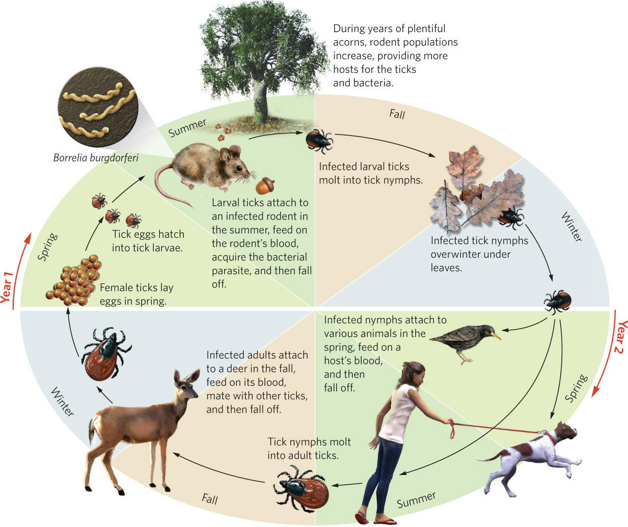
By examining patterns of abundance in nature and conducting manipulative experiments, the researchers were able to work out the life cycle of the black-legged ticks. The ticks are predominantly creatures of the forest. Larval ticks hatch from eggs each summer but since they are unable to climb very high on vegetation, they can only infect small animals living close to the ground, such as birds and rodents. The most commonly infected rodents are chipmunks (Tamias striatus) and white-footed mice (Peromyscus leucopis). These two species can be infected without exhibiting any signs of disease, so they act as reservoir species that maintain the bacterial population. After feeding on the rodents for a few days, the ticks drop off their host and molt into nymphs.
364
As nymphs, the ticks spend the winter living under the leaves on the forest floor. The following spring, they climb a short distance up in the vegetation and wait for another host to pass by. They most commonly attach to birds, small mammals, and any humans who might be taking a walk in the woods or in a garden. After attaching themselves to a host and becoming engorged with blood, the ticks drop off again and molt into adults by autumn. Adult ticks can climb higher up on vegetation, which allows them to jump onto larger mammals such as white-tailed deer. The deer’s body not only offers a blood meal but also serves as a location for adult male and female ticks to find each other and to mate. From there, they drop off the deer and lay their eggs on the forest floor each autumn. All of this movement of ticks between multiple hosts results in many opportunities for the bacteria to be transmitted. In fact, researchers found that frequency of infection with the bacteria is 25 to 35 percent for nymphs and 50 to 70 percent for adults.
Based on this research, it became clear that deer, mice, and chipmunks were keys to the tick’s life cycle. But what affects the abundances of these species? The researchers discovered one more key player: oak trees. Oak trees produce massive numbers of acorns every few years and acorns are a major food item for deer, chipmunks, and mice. In high-acorn years, tick-carrying deer gather under the oak trees, which causes an aggregation of reproducing ticks that drop their eggs under the trees. Chipmunks and mice are also attracted to the acorns since the abundant food permits higher survival and increased reproduction. More rodents and an increased density of tick eggs cause an increase in the number of infected rodents the following summer. In low-acorn years when both deer and rodents spend more time in maple forests, the prevalence of infected ticks shifts from the oak forests.
To examine what steps can be taken to reduce the risk of Lyme disease to humans, the researchers also used mathematical models that included all of the key species. These models suggested that, while reductions in deer densities would have little effect on the population of infected ticks unless the deer population were completely eradicated, reductions in the rodent population could cause a large reduction in the population of infected ticks.
The story of Lyme disease is an excellent example of how understanding the ecology of parasites allows us to predict when and where they pose the greatest risk to wild organisms and to humans.
SOURCES: Ostfeld, R. 1997. The ecology of Lyme-disease risk. American Scientist 85: 338–346.
Ostfeld, R., et al. 2006. Climate, deer, rodents, and acorns as determinants of variation in Lyme-disease risk. PLOS Biology 4: 1058–1068.