11.6 Application: Kepler's Laws of Planetary Motion

1 Discuss Kepler's Laws of Planetary Motion

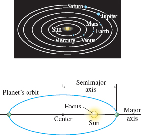
In the sixteenth century, Nicolaus Copernicus (1473–1543) proposed the Heliocentric Theory of Planetary Motion. He postulated that the planets travel in circular orbits with the Sun at the center. This theory agreed better with observation than the earlier Geocentric Theory, which claimed the Sun, moon, and planets travel in circular paths around Earth.

However, Copernicus' theory did not explain some observable facts. Early in the seventeenth century, Johannes Kepler (1571–1630) used the data of the Danish astronomer Tycho Brahe (1546–1601) to state three Laws of Planetary Motion.

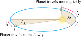
• The orbit of each planet is an ellipse with the Sun at a focus [postulated in (1609)]. See Figure 35
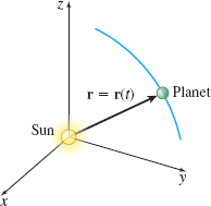
• A line joining the Sun to a planet sweeps out equal areas in equal times (1609). See Figure 36.
• The square of the period of revolution of a planet is proportional to the cube of the length of the semimajor axis of the planet's elliptical orbit (1619).

Although Kepler's Laws of Planetary Motion fit Brahe's observations, the theory could not be proved until Newton used calculus to explain the motion of planetary bodies. Here, we derive the first two of Kepler's laws using Newton's ideas and vector calculus. The proof of Kepler's third law for circular orbits is left as an exercise. See Problem 5.

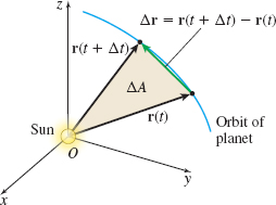
Position a coordinate system with the Sun at the origin and let \(\mathbf{r=r} (t)\) denote the position of a planet in orbit about the Sun, as shown in Figure 37. Then \(\mathbf{r}\) is subject to two laws: \begin{equation*} \begin{array}{ll@{\quad}l} \hbox{Newton's Second Law of Motion:} & & \mathbf{F}=m\mathbf{a}( t) =m\mathbf{r^{\prime \prime} }( t) \\[6pt] \hbox{Newton’s Law of Universal Gravitation:} & & \mathbf{F=-}\dfrac{GmM}{ \left\Vert \mathbf{r}\right\Vert ^{2}}\dfrac{\mathbf{r}}{\left\Vert \mathbf{r}\right\Vert } \end{array} \end{equation*}

where \(m\) is the mass of the planet, \(M\) is the mass of the Sun, \(G\) is the gravitational constant and \( \left\Vert \mathbf{r}\right\Vert \) is the distance between the Sun and the planet.

Newton's Second Law of Motion states that the force acting on an object is proportional to the acceleration of the object, its mass being the constant of proportionality. Newton's Law of Universal Gravitation states that the force \(\mathbf{F}\) of attraction between two objects of mass \(m\) and \(M\) is inversely proportional to the square of the distance between the objects and is directed along the line joining them. Here, the gravitational constant \( G~\approx 6.67\times 10^{-11}~\dfrac{\textrm{N}\,{\cdot}\, \textrm{m}^{2}}{\textrm{kg} ^{2}}\) is the constant of proportionality.

From Newton's two laws, we find \begin{equation*} \mathbf{r}^{\prime \prime} (t)=-\frac{GM}{\left\Vert \mathbf{r}\right\Vert ^{3}}\mathbf{r} \end{equation*}

If \(\mathbf{v=v}(t)\) is the velocity of a planet, then \(\mathbf{a}( t)\;=\;\dfrac{d\mathbf{v}}{dt}=\mathbf{r^{\prime \prime} }( t), \) so \begin{equation*} \bbox[5px, border:1px solid black, #F9F7ED]{\dfrac{d\mathbf{v}}{dt}=-\dfrac{GM}{\left\Vert \mathbf{r}\right\Vert ^{3}}\mathbf{r}}\tag{1} \end{equation*}

This shows that \(\dfrac{d\mathbf{v}}{dt}\) and \(\mathbf{r}\) are parallel, so \begin{equation*} \mathbf{r}\times \frac{d\mathbf{v}}{dt}=\mathbf{0} \end{equation*}

Now we differentiate \(\mathbf{r\times v}\). \begin{equation*} \frac{d}{dt} (\mathbf{r}\times \mathbf{v})=\left( \frac{d\mathbf{r}}{dt} \times \mathbf{v}\right) +\left( \mathbf{r}\times \frac{d\mathbf{v}}{dt} \right) \underset{\underset{\color{#0066A7}{\frac{d\mathbf{r}}{dt}= \mathbf{v}}}{\color{#0066A7}{\uparrow}}}{=} ( \mathbf{v}\times \mathbf{v}) +\mathbf{0}=\mathbf{0}\\ \end{equation*}

This means \(\mathbf{r}\times \mathbf{v}\) is a constant vector, which we denote by \(\mathbf{D}\). That is, \begin{equation*} \bbox[5px, border:1px solid black, #F9F7ED] {\mathbf{r}\times \mathbf{v}=\mathbf{D}}\tag{2} \end{equation*}

This fact implies that the motion of a planet lies in a plane.

We now prove Kepler's second law. A little later we prove Kepler's first law. As Figure 38 illustrates, if \(A\) is the area swept out by the vector \( \mathbf{r}\) in time \(t\), then the area \(\Delta A\) that is swept out in time \( \Delta t\) can be approximated by a triangle. Since \(\left\Vert \mathbf{r} \times \Delta \mathbf{r}\right\Vert \) is the area of a parallelogram with sides \({\bf r}\) and \(\Delta {\bf r},\) the area of the triangle is \(\dfrac{1}{2}\) the area of the parallelogram. That is, \begin{equation*} \Delta A\approx \frac{1}{2}\left\Vert \mathbf{r}\times \Delta \mathbf{r}\right\Vert \end{equation*}

and \begin{equation*} \frac{\Delta A}{\Delta t}\approx \frac{1}{2}\left\Vert \mathbf{r}\times \frac{\Delta \mathbf{r}}{\Delta t}\right\Vert \end{equation*}

As \(\Delta t\) approaches \(0\), then \(\dfrac{\Delta A}{\Delta t}\rightarrow \dfrac{dA}{dt}\) and \(\dfrac{\Delta \mathbf{r}}{\Delta t}\rightarrow \dfrac{d \mathbf{r}}{dt}.\) So, \begin{equation*} \frac{dA}{dt}=\frac{1}{2}\left\Vert \mathbf{r}\times \frac{d\mathbf{r}}{dt} \right\Vert{ \color{#0066A7}{\underset{\hbox{\(\frac{d\mathbf{r}}{dt}=\mathbf{v}\)}}{ \color{#0066A7}{\underset{{\hbox{$\uparrow$}}}{=}}}}}\frac{1}{2}\left\Vert \mathbf{r}\times \mathbf{v}\right\Vert{ \color{#0066A7}{\underset{\hbox{By (2)}}{\color{#0066A7}{\underset{{\hbox{$\uparrow$}} }{=}}}}}\frac{1}{2}\left\Vert \mathbf{D} \right\Vert \end{equation*}

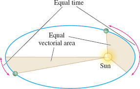
That is, \(\dfrac{dA}{dt}\) is constant. This proves Kepler's second law. See Figure 39.

To obtain Kepler's first law, we use equation (1), \(\dfrac{d\mathbf{v}}{dt}=- \dfrac{GM}{\left\Vert \mathbf{r}\right\Vert ^{3}}\mathbf{r}\), and equation (2), \(\mathbf{r }\times \mathbf{v}=\mathbf{D}\). We seek an expression for \(\dfrac{d\mathbf{ v}}{dt}\times \mathbf{D}\). \begin{equation*} \bbox[5px, border:1px solid black, #F9F7ED] {\dfrac{d\mathbf{v}}{dt}\times \mathbf{D}=-\dfrac{GM}{\left\Vert \mathbf{r} \right\Vert ^{3}}\mathbf{r}\times (\mathbf{r}\times \mathbf{v}) \underset{\underset{\color{#0066A7}{Triple Cross Product}}{\color{#0066A7}{\uparrow}}}{=} -\dfrac{GM}{\left\Vert \mathbf{r} \right\Vert ^{3}}[ (\mathbf{r}\,{\cdot}\, \mathbf{v})\mathbf{r}- (\mathbf{r} \,{\cdot}\, \mathbf{r}) \mathbf{v}]}\tag{3} \end{equation*}

Now we differentiate the dot product \(\mathbf{r}\,{\cdot}\, \mathbf{r}\). \begin{equation*} \frac{d}{dt}(\mathbf{r}\,{\cdot}\, \mathbf{r})=\frac{d\mathbf{r}}{dt}\,{\cdot}\ \mathbf{ r}+\mathbf{r}\,{\cdot}\,\frac{d\mathbf{r}}{dt}=2\mathbf{r}\,{\cdot}\, \frac{d\mathbf{r} }{dt}\underset{\underset{\color{#0066A7}{\frac{d\mathbf{r}}{dt} = \mathbf{v}}}{\color{#0066A7}{\uparrow}}}{=} 2 \mathbf{r}\,{\cdot}\, \mathbf{v}\color{#0066A7}{\hbox {}} \tag{4} \end{equation*}

Since \(\mathbf{r}\,{\cdot}\, \mathbf{r}=\left\Vert \mathbf{r}\right\Vert ^{2}\), the following is also true: \begin{equation} \frac{d}{dt}(\mathbf{r}\,{\cdot}\, \mathbf{r})=\frac{d}{dt}\left\Vert \mathbf{r} \right\Vert ^{2}=2\left\Vert \mathbf{r}\right\Vert \frac{d}{dt}\left\Vert \mathbf{r}\right\Vert \tag{5} \end{equation}

Based on (4) and (5), we have \begin{eqnarray*} 2\mathbf{r}\,{\cdot}\, \mathbf{v} &=&2\left\Vert \mathbf{r}\right\Vert \frac{d}{dt} \left\Vert \mathbf{r}\right\Vert \\[6pt] \mathbf{r}\,{\cdot}\, \mathbf{v} &=&\left\Vert \mathbf{r}\right\Vert \frac{d}{dt} \left\Vert \mathbf{r}\right\Vert \end{eqnarray*}

We substitute this result in (3). Then \begin{eqnarray*} \frac{d\mathbf{v}}{dt}\times \mathbf{D}&=&-\frac{GM}{\left\Vert \mathbf{r}\right\Vert ^{3} }\left[ (\mathbf{r}\,{\cdot}\, \mathbf{v})\mathbf{r}-(\mathbf{r}\,{\cdot}\, \mathbf{r}) \mathbf{v}\right]\;=\;-\frac{GM}{\left\Vert \mathbf{r}\right\Vert ^{3}}\left[ \left\Vert \mathbf{r}\right\Vert \left( \frac{d}{dt}\left\Vert \mathbf{r}\right\Vert \right) \mathbf{r}-\left\Vert \mathbf{r}\right\Vert ^{2}\mathbf{v}\right]\\[6pt] &=&GM\left( \frac{\mathbf{v}}{\left\Vert \mathbf{r}\right\Vert }-\frac{\mathbf{r}}{\left\Vert \mathbf{r} \right\Vert ^{2}}\frac{d}{dt}\left\Vert \mathbf{r}\right\Vert \right) \end{eqnarray*}

But, \begin{equation*} \frac{d}{dt}\frac{\mathbf{r}}{\left\Vert \mathbf{r}\right\Vert }=\frac{\dfrac{d\mathbf{r }}{dt}}{\left\Vert \mathbf{r}\right\Vert }-\frac{\mathbf{r}}{\left\Vert \mathbf{r}\right\Vert ^{2}} \frac{d}{dt}\left\Vert \mathbf{r}\right\Vert\;=\;\frac{\mathbf{v}}{\left\Vert \mathbf{r}\right\Vert }- \frac{\mathbf{r}}{\left\Vert \mathbf{r}\right\Vert ^{2}}\frac{d}{dt}\left\Vert \mathbf{r} \right\Vert \end{equation*}

As a result, we can write \begin{equation*} \dfrac{d\mathbf{v}}{dt}\times \mathbf{D}=GM\left( \dfrac{d}{dt}\dfrac{ \mathbf{r}}{\left\Vert \mathbf{r}\right\Vert }\right) \end{equation*}

Since \(\mathbf{D}\) is a constant vector, we can integrate both sides and obtain \begin{equation*} \mathbf{v}\times \mathbf{D}=GM\frac{\mathbf{r}}{\left\Vert \mathbf{r}\right\Vert }+ \mathbf{H} \end{equation*}

where \(\mathbf{H}\) is a constant vector.

To find \(\left\Vert \mathbf{r}\right\Vert \), we first find the dot product \( \mathbf{r}\,{\cdot}\, ( \mathbf{v\times D}) \): \begin{equation*} \mathbf{r}\,{\cdot}\, (\mathbf{v}\times \mathbf{D})=\mathbf{r\,{\cdot} }\left( GM \dfrac{\mathbf{r}}{\left\Vert \mathbf{r}\right\Vert }+\mathbf{H}\right) =GM\left\Vert \mathbf{r}\right\Vert +\mathbf{r}\,{\cdot}\, \mathbf{H} \end{equation*}

But \(\mathbf{A}\,{\cdot}\, (\mathbf{B}\times \mathbf{C})=(\mathbf{A}\times \mathbf{ B})\,{\cdot}\, \mathbf{C}\), so \begin{equation*} (\mathbf{r}\times \mathbf{v})\,{\cdot}\, \mathbf{D}=GM\left\Vert \mathbf{r}\right\Vert + \mathbf{r}\,{\cdot}\, \mathbf{H} \end{equation*}

Since \(\mathbf{r}\times \mathbf{v}=\mathbf{D}\), we have \begin{equation*} \left\Vert \mathbf{D}\right\Vert ^{2}=GM\left\Vert \mathbf{r}\right\Vert +\mathbf{r}\,{\cdot}\, \mathbf{H} \end{equation*}

If \(\theta \) is the angle between \(\mathbf{r}\) and \(\mathbf{H}\), then \(\cos \theta\;=\;\dfrac{\mathbf{r}\,{\cdot}\, \mathbf{H}}{\left\Vert \mathbf{r}\right\Vert \left\Vert \mathbf{H}\right\Vert },\) so \begin{equation*} \left\Vert \mathbf{D}\right\Vert ^{2}=GM\left\Vert \mathbf{r}\right\Vert +\left\Vert \mathbf{r} \right\Vert \left\Vert \mathbf{H}\right\Vert \cos \theta \end{equation*}

Now we solve for \(\left\Vert \mathbf{r}\right\Vert \): \begin{equation*} \left\Vert \mathbf{r}\right\Vert\;=\;\frac{\left\Vert \mathbf{D}\right\Vert ^{2}}{GM+\left\Vert \mathbf{H} \right\Vert \cos \theta }=\frac{\left\Vert \mathbf{D}\right\Vert ^{2}}{GM}\left( \frac{1}{ 1+e\cos \theta }\right) \end{equation*}

where \(e=\dfrac{\left\Vert \mathbf{H}\right\Vert }{GM}\). This is the polar equation of a conic with a focus at the origin, the Sun. It is a hyperbola if \(e>1\), a parabola if \(e=1\), or an ellipse if \(e <1\). Since the planets have closed orbits, the only possibility is an ellipse, resulting in Kepler's First Law of Planetary Motion: