11.3 Arc Length as Parameter; CurvaturePrinted Page 774
OBJECTIVES
When you finish this section, you should be able to:
In this section, we discuss geometric properties of curves.
We have seen that the same curve can be defined using different parametric equations. For example, the upper half of a unit circle can be given by \begin{equation*} \mathbf{r}(t)=t\mathbf{i}+\sqrt{1-t^{2}}\mathbf{j}\quad -\!1\leq t\leq 1 \end{equation*}
where \(x( t) =t\) and \(y( t) =\sqrt{1-t^{2}}\). Here, the parameter \(t\) is the position on the \(x\)-axis.
This same curve can be given by \begin{equation*} \mathbf{r}(t)=\cos t\mathbf{i}+\sin t\mathbf{j}\quad 0\leq t\leq \pi \end{equation*}
where \(x( t) =\cos t\) and \(y( t) =\sin t\). Here, the parameter \(t\) is the angle between the positive \(x\)-axis and \(\mathbf{r}=\mathbf{r}( t) \). Since the curve is the upper half of the unit circle, the arc length \(s\) subtended by the angle \(t\) is \(s=r\theta =t.\) That is, the parameter \(t\) equals the arc length along the circle.
Just as time is the preferred parameter for motion along a curve, arc length along a curve is the preferred parameter for discussing a curve's geometric properties—for several reasons.
775
First, the arc length of a curve is a natural consequence of the curve's shape. Further, arc length is independent of the representation of the curve. For example, the arc length of the semi-circle, \(x=2t,\) \(y=2\sqrt{1-t^{2}},\) \(-1\leq t\leq 1\), is \(2\pi .\) The arc length of the same semi-circle, \(x=2\sin\theta, \) \(y=2\cos \theta, \) \(-\dfrac{\pi }{2}\leq \theta \leq \dfrac{\pi }{2}\), is also \(2\pi\). No matter how the curve is defined, its arc length is the same.
1 Determine Whether the Parameter Used in a Vector Function Is Arc LengthPrinted Page 775
So how do we determine whether the parameter of a curve represents arc length? And, if it doesn't, how can we change the parameter so it does represent arc length? The next result provides a means for determining whether the parameter of a vector function is arc length.
Let's examine the relationship between arc length \(s\) along a curve \(C\) and the parameter \(t\) used to define \(C.\) The arc length \(s\) of a smooth curve \(C\) traced out by a vector function \(\mathbf{r}=\mathbf{r}(t),\) \(a\leq t\leq b\), from \(a\) to an arbitrary parameter value \(t\) in \(\left[ a,b\right]\) is \begin{equation} s(t)=\int_{a}^{t}\left\Vert \mathbf{r}^{\prime} (u)\right\Vert du \tag{1} \end{equation}
Then, by the Fundamental Theorem of Calculus, \begin{equation*} \bbox[5px, border:1px solid black, #F9F7ED] {\dfrac{ds}{dt}\;=\;\left\Vert \mathbf{r}^{\prime }(t)\right\Vert }\tag{2} \end{equation*}
THEOREM Criterion for Arc Length as Parameter
Suppose a smooth curve \(C\) is traced out by the vector function \begin{equation*} \mathbf{r}=\mathbf{r}(t)\quad a\leq t\leq b \end{equation*}
The parameter \(t\) is the arc length along \(C\) if and only if \begin{equation*} \bbox[5px, border:1px solid black, #F9F7ED] {\left\Vert \mathbf{r}^{\prime} (t)\right\Vert\;=\;1\quad \hbox{for all}\quad t} \end{equation*}
Proof
We use equation (1). If \(\left\Vert \mathbf{r}^{\prime} (t)\right\Vert\;=\;1\) for all \(t,\) then the arc length \(s\) is \begin{equation*} s(t)=\int_{a}^{t}du=t-a \end{equation*}
That is, the parameter \(t\) is the arc length \(s\) measured along \(C\) from \(t = a\) to \(t= b\). Notice that when \(t=a,\) the length \(s\) is zero, as expected.
Conversely, if the parameter \(t\) is arc length \(s\), then, by differentiating (1), we obtain \[ \frac{ds}{dt}=1=\;\left\Vert \mathbf{r}^{\prime }(t)\right\Vert\qquad \hbox{for all}\quad t \]
EXAMPLE 1Determining Whether the Parameter Used in a Vector Function Is Arc Length
Determine whether the parameter used in each vector function is arc length.
(a) \(C_{1}\): \(\ \mathbf{r}(t)=2\sin \dfrac{t}{2}\mathbf{i}+2\cos \dfrac{t}{2}\mathbf{j}\quad 0\leq t\leq 2\pi \)
(b) \(C_{2}\): \(\ \mathbf{r}(t)=\cos t\mathbf{i}+\sin t\mathbf{j}+t\mathbf{k}\quad t\geq 0\)
Solution (a) We begin by finding \(\mathbf{r}^{\prime} ( t)\) and \(\left\Vert \mathbf{r^{\prime} }( t) \right\Vert .\) \begin{equation*} \begin{array}{rrr} \mathbf{r}^{\prime} (t)=\cos \dfrac{t}{2}\mathbf{i}-\sin \dfrac{t}{2}\mathbf{j} \qquad \left\Vert \mathbf{r}^{\prime} (t)\right\Vert\;=\;\sqrt{ \cos ^{2}\dfrac{t}{2}+\sin ^{2}\dfrac{t}{2}}=1\quad \hbox{for all}~t \end{array} \end{equation*}
776
Since \(\left\Vert \mathbf{r}^{\prime} (t)\right\Vert\;=\;1\) for all \(t,\) the parameter \(t\) is arc length as measured along \(C_{1}\).
(b) We begin by finding \(\mathbf{r}^{\prime} ( t)\) and \(\left\Vert \mathbf{r^{\prime} }( t) \right\Vert .\) \begin{equation*} \begin{array}{rrr} \mathbf{r}^{\prime} (t)=-\sin t\mathbf{i}+\cos t\mathbf{j+k}\qquad \left\Vert \mathbf{r}^{\prime} (t)\right\Vert\;=\;\sqrt{\sin ^{2}t+\cos ^{2}t+1}=\sqrt{2} \end{array} \end{equation*}
Since \(\left\Vert \mathbf{r}^{\prime }(t)\right\Vert\;\neq 1\) for all \(t\), the parameter \(t\) does not measure arc length along \(C_{2}\).
NOW WORK
EXAMPLE 2Changing the Parameter to Arc Length
Represent the helix in Example 1(b). \begin{equation*} \mathbf{r}(t)=\cos t\mathbf{i}+\sin t\mathbf{j}+t\mathbf{k}\quad t\geq 0 \end{equation*}
so the parameter is arc length.
Solution The arc length function \(s( t)\) along the curve \(\mathbf{r}=\mathbf{r}( t)\), \(a\leq t\leq b\), from \(t=a\) to an arbitrary \(t\) is given by the integral \begin{equation*} s( t)\;=\;\int_{a}^{t}\left\Vert \mathbf{r}^{\prime} (u)\right\Vert du \end{equation*}
Since the graph of the helix starts at \(t=0,\) and \(\left\Vert \mathbf{r}^{\prime}(t)\right\Vert\;=\;\sqrt{2}\) for all \(t\) (Example 1(b)), we have \begin{equation*} s( t)\;=\;\int_{0}^{t}\sqrt{2}\kern.7ptdu=\Big[ \sqrt{2}\kern.7ptu\Big] _{0}^{t}= \sqrt{2}\kern.7pt t \end{equation*}
Then \(t=\dfrac{s}{\sqrt{2}}.\) The helix using arc length \(s\) as the parameter is expressed as \begin{equation*} \mathbf{r}( s)\;=\;\cos \dfrac{s}{\sqrt{2}}\kern.7pt\mathbf{i}+\sin \dfrac{s}{ \sqrt{2}}\kern.7pt\mathbf{j}+\dfrac{s}{\sqrt{2}}\kern.7pt\mathbf{k}\quad s\geq 0 \end{equation*}
As Example 2 shows, to change the parameter \(t\) of a curve \(C\) traced out by the vector function \(\mathbf{r}=\mathbf{r}( t)\), \(a\leq t\leq b,\) to arc length \(s\) requires finding the integral \begin{equation*} s( t)\;=\;\int_{a}^{t}\left\Vert \mathbf{r}^{\prime} ( u) \right\Vert du \end{equation*}
Since \(\left\Vert \mathbf{r}^{\prime} ( u) \right\Vert\) is continuous on \(( a,b)\) and \(\mathbf{r}^{\prime} ( t)\) is never zero on \(( a,b)\), then \(s=s( t)\) exists for all \(t\geq a.\) Moreover, \(s^{\prime} ( t)\;=\;\left\Vert \mathbf{r}^{\prime} ( t) \right\Vert >0,\) so \(s\) is increasing and has an inverse function. To find it, we need to solve \(s=s( t)\) for \(t.\) For most curves, finding the integral and solving for \(t\) is not possible. Regardless, for smooth curves, we know an arc length parameterization exists. In the discussion that follows, we make use of this fact and assume the curve is expressed using arc length as the parameter.
2 Find the Curvature of a CurvePrinted Page 778
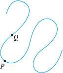
A curve may change direction quickly at some points and slowly at others. For example, the curve in Figure 19 bends sharply at \(P,\) but at \(Q\) the curve bends only a little. Curvature is a measure of how sharply a curve bends, that is, curvature measures how much the direction of the curve is changing. For the curve in Figure 19, the curvature at \(P\) is greater than the curvature at \(Q\).
The amount a curve changes direction at a point can be quantified using the unit tangent vector \(\mathbf{T}\) at the point. If we move a little away from \(Q\) and there is little or no change in the direction of \(\mathbf{T}\), the curve has not bent much. If we move a little away from \(P\) and the direction of \(\mathbf{T}\) changes dramatically, the curve has bent a lot. The curvature of \(C\) at \(Q\) is less than the curvature at \(P\) because the tangent vectors near \(P\) have turned more than the tangent vectors near \(Q.\) We use the rate of change of the tangent vectors to measure curvature.
777
NOTE
\(k\) is the Greek letter kappa.
DEFINITION Curvature
Suppose a smooth curve \(C\) is traced out by a twice differentiable vector function \(\mathbf{r}=\mathbf{r}(s)\), where the parameter is the arc length \(s\) along \(C\). The curvature \(\kappa\;=\;\kappa (s)\) at a point \(P\) on \(C\) is \begin{equation*} \bbox[5px, border:1px solid black, #F9F7ED] {\kappa\;=\;\left\Vert \dfrac{d\mathbf{T}}{ds}\right\Vert} \end{equation*}
IN WORDS
Curvature is measured by the magnitude of the rate of change of the unit tangent vector \(\mathbf{T}\) with respect to arc length.
In the next example, we find the curvature of a line. Since a line has constant direction, the tangent vectors never turn so the curvature of the line is \(0.\)
EXAMPLE 3Finding the Curvature of a Line
Show that the curvature of a line is \(0\).
Solution For a line, the unit tangent vector \(\mathbf{T}\) is along the constant direction of the line, so \(\mathbf{T}\) is a constant and \(\dfrac{d\mathbf{T}}{ds}=\mathbf{0}\). The curvature \(\kappa\;=\;\left\Vert \dfrac{d\mathbf{T}}{ds}\right\Vert\) of a line is \(0\).
As we stated earlier, it is not easy to express a curve using arc length as the parameter. So, we seek expressions for the curvature \(\kappa\) that do not require the parameter to be arc length. Suppose \(\mathbf{T}=\mathbf{T}( t)\) is the unit tangent vector of a curve \(C\) traced out by the vector function \(\mathbf{r}=\mathbf{r}( t),\) \(a\leq t\leq b.\) If \(s\) is the arc length along \(C,\) then we can use the Chain Rule to obtain \begin{equation*} \dfrac{d\mathbf{T}}{dt}=\dfrac{d\mathbf{T}}{ds}\dfrac{ds}{dt} \end{equation*}
Since \(\dfrac{ds}{dt}\;=\;\left\Vert \mathbf{r}^{\prime} (t) \right\Vert\;\neq 0,\) then \begin{equation*} \kappa\;=\;\left\Vert \dfrac{d\mathbf{T}}{ds}\right\Vert\;=\;\left\Vert \dfrac{ \mathbf{T}^{\prime} (t) }{\dfrac{ds}{dt}}\right\Vert \end{equation*}
Since \(\dfrac{ds}{dt}\;=\;\left\Vert \mathbf{r}^{\prime} (t) \right\Vert\), we have the following expression for the curvature \(\kappa\) of a curve \(C\) in terms of any parameterization of \(C\): \begin{equation*} \bbox[5px, border:1px solid black, #F9F7ED] {\kappa\;=\;\dfrac{\left\Vert \mathbf{T}^{\prime} (t) \right\Vert }{\left\Vert \mathbf{r}^{\prime} (t) \right\Vert}} \tag{3} \end{equation*}
The next example finds the curvature of a circle. Since a circle has a tangent line that turns uniformly, its curvature is a constant. What that constant is may surprise you.
EXAMPLE 4Finding the Curvature of a Circle
Find the curvature of a circle of radius \(R.\)
Solution For a circle of radius \(R,\) \begin{equation*} \mathbf{r}=\mathbf{r}( t)\;=\;R\;\cos t\mathbf{i}+R\;\sin t\mathbf{j}\qquad 0\leq t\leq 2\pi \end{equation*}
Then we find \(\mathbf{r}^{\prime} (t)\) and \(\left\Vert \mathbf{r^{\prime} }(t) \right\Vert.\) \begin{equation*} \begin{array}{rrr} \mathbf{r}^{\prime} ( t)\;=\;-R\;\sin t\mathbf{i}+R\;\cos t\mathbf{j}\qquad \Vert \mathbf{r}^{\prime} (t) \Vert\;=\;\sqrt{R^{2}\sin ^{2}t+R^{2}\cos ^{2}t}=R \end{array} \end{equation*}
778
The unit tangent vector \(\mathbf{T}\) and its derivative \(\mathbf{T^{\prime} }\) are \begin{eqnarray*} \mathbf{T}(t) &=&\dfrac{\mathbf{r}^{\prime} (t) }{ \left\Vert \mathbf{r}^{\prime} (t) \right\Vert }=\dfrac{-R\;\sin t \mathbf{i}+R\;\cos t\mathbf{j}}{R}=-\sin t\mathbf{i}+\cos t\mathbf{j} \\[6pt] \mathbf{T}^{\prime} (t) &=&-\cos t\mathbf{i}-\sin t\mathbf{j}\qquad \left\Vert \mathbf{T^{\prime} }(t) \right\Vert\;=\;1 \end{eqnarray*}
We use formula (3) to find the curvature \(\kappa\). \begin{equation*} \kappa\;=\;\dfrac{\left\Vert \mathbf{T}^{\prime} (t) \right\Vert }{ \left\Vert \mathbf{r}^{\prime} (t) \right\Vert }=\dfrac{1}{R} \end{equation*}
NOTE
The larger a circle, the smaller its curvature. As \(R\rightarrow \infty\), then \(\kappa \rightarrow 0\). and the circle will look more and more like a line.
The curvature of a circle of radius \(R\) is the reciprocal of its radius.
NOW WORK
3 Find the Curvature of a Space CurvePrinted Page 778
It is easier to find the curvature of a curve in space using the following formula rather than (3).
THEOREM Curvature of a Space Curve
If a smooth curve \(C\) in space is traced out by a twice differentiable vector function \(\mathbf{r}=\mathbf{r}(t),\) then its curvature \(\kappa\) is given by the formula \begin{equation*} \bbox[5px, border:1px solid black, #F9F7ED] {\kappa\;=\;\dfrac{\left\Vert \mathbf{r}^{\prime} (t)\times \mathbf{r}^{\prime \prime} (t)\right\Vert }{\left\Vert \mathbf{r}^{\prime} (t) \right\Vert ^{3}}} \tag{4} \end{equation*}
NEED TO REVIEW?
The cross product and its properties are discussed in Section 10.5, pp. 724-729.
Proof
Since \(\mathbf{T}(t)\;=\;\dfrac{\mathbf{r}^{\prime} (t)}{ \left\Vert \mathbf{r}^{\prime} (t)\right\Vert }\) and \( \left\Vert \mathbf{r} ^{\prime} (t)\right\Vert\;=\;\dfrac{ds}{dt}\) [from (2) on p. 775], then \begin{equation} \mathbf{r}^{\prime} (t)\;=\;\left\Vert \mathbf{r}^{\prime} (t)\right\Vert\kern1pt\mathbf{T} (t)\;=\frac{ds}{dt}\kern1pt\mathbf{T}(t) \tag{5} \end{equation}
Now we use the scalar multiplication formula to find \(\mathbf{r^{\prime\prime}} (t)\). \begin{equation} \mathbf{r}^{\prime \prime} (t)=\dfrac{d}{dt}\kern1pt\mathbf{r}^{\prime} (t)=\frac{d}{dt} \left( \frac{ds}{dt}\kern1pt\mathbf{T}(t)\right)\;=\;\frac{d^{2}s}{dt^{2}}\kern1pt\mathbf{T} (t)+\frac{ds}{dt}\kern1pt\mathbf{T}^{\prime} (t) \tag{6} \end{equation}
Using (5) and (6), we get \begin{equation*} \mathbf{r}^{\prime} (t) \times \mathbf{r}^{\prime \prime} (t)\;=\;\dfrac{ds}{dt}\kern1pt\mathbf{T}\times \left( \frac{d^{2}s}{dt^{2}}\kern1pt \mathbf{T}+\frac{ds}{dt}\kern1pt\mathbf{T}^{\prime} \right)\;=\;\dfrac{ds}{dt} \frac{d^{2}s}{dt^{2}} \left( \mathbf{T}\times \mathbf{T}\right) +\left( \dfrac{ds}{dt}\right) ^{2}\left( \mathbf{T}\times \mathbf{T}^{\prime} \right) \end{equation*}
Since \(\mathbf{T}\times \mathbf{T}=\mathbf{0}\), this reduces to \begin{equation} \mathbf{r}^{\prime} (t) \times \mathbf{r}^{\prime \prime} (t)\;=\;\left( \dfrac{ds}{dt}\right)^{2}\left( \mathbf{T}\times \mathbf{T}^{\prime} \right) \tag{7} \end{equation}
RECALL
\(\left\Vert \mathbf{u}\times \mathbf{v} \right\Vert\;=\;\left\Vert \mathbf{u}\right\Vert \left\Vert \mathbf{v}\right\Vert \sin\theta\), where \(\theta\) is the angle between \(\mathbf{u}\) and \(\mathbf{v}.\)
Since \(\mathbf{T^{\prime} }\) is parallel to \(\mathbf{N}\) and \(\mathbf{T}\) is orthogonal to \(\mathbf{N}\), it follows that \(\mathbf{T}\) and \(\mathbf{T}^{\prime}\) are orthogonal. This means \(\left\Vert \mathbf{T}\times \mathbf{T}^{\prime} \right\Vert\;=\;\left\Vert \mathbf{T}\right\Vert \left\Vert \mathbf{T}^{\prime} \right\Vert \sin \dfrac{\pi }{2}\;=\left\Vert \mathbf{T}^{\prime} \right\Vert\), so \begin{equation*} \left\Vert \mathbf{r}^{\prime} (t) \times \mathbf{r}^{\prime \prime} (t) \right\Vert\;=\;\left( \dfrac{ds}{dt}\right) ^{2}\left\Vert \mathbf{T}^{\prime} \right\Vert \end{equation*}
Now we solve the above equation for \(\left\Vert \mathbf{T}^{\prime} \right\Vert\) and use the fact that \(\dfrac{ds}{dt}=\;\left\Vert \mathbf{r}^{\prime} (t) \right\Vert.\) Then \begin{equation} \left\Vert \mathbf{T}^{\prime} \right\Vert\;=\;\dfrac{\left\Vert \mathbf{r}^{\prime} (t) \times \mathbf{r}^{\prime \prime} (t) \right\Vert }{ \left\Vert \mathbf{r}^{\prime} (t) \right\Vert ^{2}} \tag{8} \end{equation}
From equation (3), the curvature \(\kappa\) is \begin{equation} \kappa \underset{\underset{\color{#0066A7}{\hbox{\((3)\)}}}{\color{#0066A7}{\uparrow}}}{=}\dfrac{\left\Vert \mathbf{T}^{\prime} \right\Vert }{\left\Vert \mathbf{r}^{\prime} (t) \right\Vert } \underset{\underset{\color{#0066A7}{\hbox{\((8)\)}}}{\color{#0066A7}{\uparrow}}}{=}\dfrac{\left\Vert \mathbf{r}^{\prime} (t) \times \mathbf{r}^{\prime \prime} (t) \right\Vert }{\left\Vert \mathbf{r}^{\prime} (t) \right\Vert ^{3}} \notag \end{equation}
779

EXAMPLE 5Finding the Curvature of a Space Curve
Find the curvature \(\kappa\) of the space curve \(\mathbf{r}(t)=t\mathbf{i}+t^{2}\mathbf{j}+t^{3}\mathbf{k}\).
Solution To use formula (4), we need to find \(\mathbf{r}^{\prime} (t),\) \(\left\Vert \mathbf{r}^{\prime} (t) \right\Vert,\) \(\mathbf{r}^{\prime \prime} (t),\) \(\mathbf{r}^{\prime} (t) \times \mathbf{r}^{\prime \prime} (t),\) and \(\left\Vert \mathbf{r}^{\prime} (t) \times \mathbf{r}^{\prime \prime} (t) \right\Vert.\) \begin{eqnarray*} \mathbf{r}^{\prime} (t) &=&\mathbf{i}+2t\mathbf{j}+3t^{2}\mathbf{k}\qquad \left\Vert \mathbf{r}^{\prime} (t)\right\Vert\;=\;\sqrt{ 1+4t^{2}+9t^{4}}\\ \mathbf{r}^{\prime \prime} (t) &=&2\mathbf{j}+6t\mathbf{k} \end{eqnarray*} \begin{eqnarray*} \mathbf{r}^{\prime} (t)\times \mathbf{r}^{\prime \prime} (t)&\;=\;&\left\vert \begin{array}{c@{\quad}c@{\quad}c} \mathbf{i} & \mathbf{j} & \mathbf{k} \\[3pt] 1 & 2t & 3t^{2}\\ 0 & 2 & 6t \end{array} \right\vert\;=\;6t^{2}\mathbf{i}-6t\mathbf{j}+2\mathbf{k} \\[6pt] \left\Vert \mathbf{r}^{\prime} (t)\times \mathbf{r}^{\prime \prime} (t)\right\Vert &\;=\;&\sqrt{36t^{4}+36t^{2}+4}=2\sqrt{9t^{4}+9t^{2}+1} \end{eqnarray*}
Now we use formula (4). The curvature \(\kappa\) is \begin{equation*} \kappa\;=\;\dfrac{\left\Vert \mathbf{r}^{\prime} (t)\times \mathbf{r}^{\prime \prime} (t)\right\Vert }{\left\Vert \mathbf{r}^{\prime} (t) \right\Vert ^{3}}=\frac{2\sqrt{ 9t^{4}+9t^{2}+1}}{(1+4t^{2}+9t^{4})^{3/2}} \end{equation*}
NOW WORK
4 Find the Curvature of a Plane Curve Given by \(y=f(x)\)Printed Page 779
The curvature formula \(\kappa\;=\;\dfrac{\left\Vert \mathbf{r}^{\prime} (t) \times \mathbf{r}^{\prime \prime} (t) \right\Vert }{\left\Vert \mathbf{r}^{\prime} (t) \right\Vert ^{3}}\) for a space curve can be used to find the curvature of a plane curve given by a twice differentiable function \(y=f(x)\). We use \(x\) as the parameter and define the plane curve \(y=f(x)\) using the vector equation \begin{equation*} \mathbf{r}=\mathbf{r}( x)\;=\;x\kern.7pt\mathbf{i}+f( x) \kern.7pt\mathbf{j} +0\kern.7pt\mathbf{k} \end{equation*}
Notice that a \(\mathbf{k}\)-component of \(0\) is used. Then \begin{eqnarray*} \mathbf{r}^{\prime} ( x) &=&\mathbf{i}+f^{\prime} ( x) \mathbf{j}\qquad \left\Vert \mathbf{r}^{\prime} ( x) \right\Vert\;=\;\sqrt{1+[ f^{\prime} ( x) ] ^{2}} \\[3pt] \mathbf{r}^{\prime \prime} ( x) &=&f^{\prime \prime} ( x) \mathbf{j} \\[6pt] \mathbf{r}^{\prime} ( x) \times \mathbf{r}^{\prime \prime} ( x) &=& \left|\begin{array}{c@{\quad}c@{\quad}c} \mathbf{i} & \mathbf{j} & \mathbf{k} \\[3pt] 1 & f^{\prime} ( x) & 0 \\[3pt] 0 & f^{\prime \prime} ( x) & 0 \end{array}\right| =f^{\prime \prime} ( x) \mathbf{k} \end{eqnarray*}
Now we use formula (4). \begin{equation*} \bbox[5px, border:1px solid black, #F9F7ED] {\kappa\;=\;\dfrac{\left\Vert \mathbf{r}^{\prime} (x) \times \mathbf{r}^{\prime \prime} (x) \right\Vert }{ \left\Vert \mathbf{r}^{\prime} (x) \right\Vert ^{3}}=\dfrac{ \vert f^{\prime \prime} (x) \vert }{( 1+[ f^{\prime} (x) ] ^{2}) ^{3/2}}} \tag{9} \end{equation*}
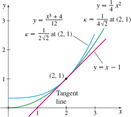
EXAMPLE 6Finding the Curvature of Plane Curves
(a) Find an equation of the tangent line to the graph of the parabola \(f(x)\;=\;\dfrac{1}{4}x^{2}\) at the point \((2,1).\)
(b) What is the curvature of the graph of \(f\) at the point \((2,1)?\)
(c) Find an equation of the tangent line to the graph of \(g(x)\;=\;\dfrac{x^{3}+4}{12}\) at the point \((2,1).\)
(d) What is the curvature of the graph of \(g\) at the point \(( 2,1)?\)
(e) Graph both curves and their tangent lines.
780
Solution (a) \(f(x)\;=\;\dfrac{1}{4}x^{2};\) \(f^{\prime} (x)\;=\;\dfrac{1}{2}x\). An equation of the tangent line to the graph of \(f\) at the point \(( 2,1)\) is \begin{eqnarray*} y-1 &=&1\,{\cdot}\, (x-2)\qquad \color{#0066A7}{f^{\prime} (2)\;=\;{1}} \\[4pt] y &=&x-1 \end{eqnarray*}
(b) \(f^{\prime \prime} (x)\;=\;\dfrac{1}{2};\quad f^{\prime} (2)\;=\;1;\quad f^{\prime \prime} (2)\;=\;\dfrac{1}{2}\). We use formula (9) and evaluate \(\kappa\) at \(x=2\). \begin{equation*} \kappa\;=\;\dfrac{\left\vert f^{\prime \prime} ( 2) \right\vert }{ \left( 1+\left[ f^{\prime} ( 2) \right] ^{2}\right) ^{3/2}}=\dfrac{ \dfrac{1}{2}}{( 1+1) ^{3/2}}=\dfrac{1}{2\,{\cdot}\, 2\sqrt{2}}=\dfrac{1 }{4\sqrt{2}}\approx 0.177 \end{equation*}
(c) \(g(x)\;=\;\dfrac{x^{3}+4}{12};\quad g^{\prime} (x)\;=\;\dfrac{3x^{2}}{12}=\dfrac{x^{2}}{4}\). An equation of the tangent line to the graph of \(g\) at the point \((2,1)\) is \begin{eqnarray*} y-1 &=&1\,{\cdot}\, ( x-2)\qquad \color{#0066A7}{g^{\prime} (2)\;=\;{1}} \\[4pt] y &=&x-1 \end{eqnarray*}
(d) \(g^{\prime \prime} (x)\;=\;\dfrac{x}{2};\quad g^{\prime} (2)\;=\;1;\quad g^{\prime \prime} (2)\;=\;1\). The curvature \(\kappa\) at the point \((2,1)\) is \begin{equation*} \kappa\;=\;\dfrac{\vert g^{\prime \prime} ( 2) \vert }{ ( 1+[ g^{\prime} ( 2) ] ^{2}) ^{3/2}}=\dfrac{1 }{( 1+1) ^{3/2}}=\dfrac{1}{2\sqrt{2}}\approx 0.354 \end{equation*}
(e) The functions \(f\) and \(g\) are graphed in Figure 20. Both graphs have the same tangent line at \((2,1),\) but the tangent line to the graph of \(y=\dfrac{1}{4}x^{2}\) at \((2,1)\) turns more slowly \((\kappa \approx 0.177)\) than the tangent line to the graph of \(y=\dfrac{x^{3}+4}{12}\) at \((2,1)\) \((\kappa \approx 0.354)\).
NOW WORK
5 Find an Osculating CirclePrinted Page 780
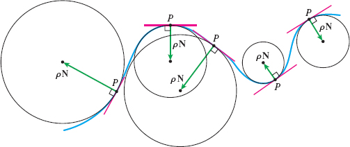
Provided the curvature \(\kappa \neq 0,\) each point \(P\) on a smooth curve \(C\) traced out by a twice differentiable vector function \(\mathbf{r=r}(t)\) can be associated with a circle, called the osculating circle of \(C\) at \(P.\) The osculating circle of \(C\) at \(P\) has the following properties:
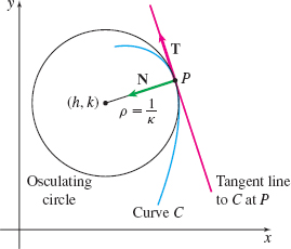
- The osculating circle contains the point \(P\).
- The tangent line to \(C\) at \(P\) and the tangent line to the osculating circle at \(P\) are the same.
- The radius \(\rho\) of the osculating circle is \(\rho\;=\;\dfrac{1}{\kappa},\) where \(\kappa\) is the curvature of \(C\) at \(P.\) That is, the osculating circle and the curve \(C\) have the same curvature at \(P.\)
- The center of the osculating circle lies on a line in the direction of the principal unit normal \(\mathbf{N}\) to \(C\) at the point \(P\).
Figure 21 illustrates these properties.
NOTE
The term osculating means “kissing.”
The osculating circle of a curve \(C\) is sometimes called the circle of curvature. Its radius \(\rho\;=\;\dfrac{1}{\kappa}\) is called the radius of curvature, and its center is called the center of curvature.
781
Since the osculating circle and the curve share a common tangent at each point and have the same curvature at each point, sometimes the osculating circle is used to approximate the curve \(C\). See Figure 22.
NOTE
The osculating circle at a point \(P\) is the limiting circle that results from the circle containing three points \(P,Q\), and \(R\) on the curve \(C\) as the points \(Q\) and \(R\) are made to approach point \(P\).


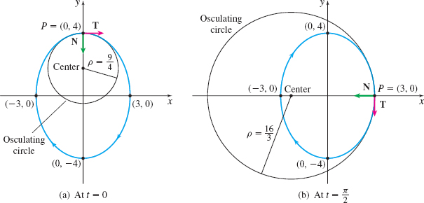
EXAMPLE 7Finding an Osculating Circle for an Ellipse
Find the radius of the osculating circle of the ellipse traced out by the vector function \begin{equation*} \mathbf{r}(t)=3\sin t\mathbf{i}+4\cos t\mathbf{j} \qquad 0\leq t\leq 2\pi \end{equation*}
(a) At \(t=0\)
(b) At \(t=\dfrac{\pi }{2}\)
Solution To find the radius of the osculating circle, we need to find the curvature \(\kappa\). We treat the ellipse as a curve in space with a \(\mathbf{k}\) component of \(0\) and find \(\mathbf{r}^{\prime} (t),\) \(\left\Vert \mathbf{r}^{\prime} (t) \right\Vert, \mathbf{r}^{\prime \prime} (t),\) \(\mathbf{r}^{\prime} (t) \times \mathbf{r}^{\prime \prime} (t),\) and \(\left\Vert \mathbf{r}^{\prime} (t) \times \mathbf{r}^{\prime \prime} (t) \right\Vert\). \begin{eqnarray*} \mathbf{r^{\prime} }(t) &=& 3\cos t\mathbf{i}-4\sin t\mathbf{j}+0\mathbf{k} \qquad \left\Vert \mathbf{r^{\prime} }(t) \right\Vert\;=\; \sqrt{9\cos ^{2}t+16\sin ^{2}t}\\[9pt] \mathbf{r^{\prime \prime} }(t) &=& -3\sin t\mathbf{i}-4\cos t\mathbf{j}+0\mathbf{k} \end{eqnarray*}
\begin{eqnarray*} \mathbf{r^{\prime} }(t)\times \mathbf{r^{\prime \prime} }(t)= \left|\begin{array}{c@{\quad}c@{\quad}c} \mathbf{i} & \mathbf{j} & \mathbf{k} \\[3pt] 3\cos t & -4\sin t & 0 \\[3pt] -3\sin t & -4\cos t & 0 \end{array}\right| &=&( -12\cos ^{2}t-12\sin ^{2}t) \mathbf{k}=-12\mathbf{k}\\[9pt] \left\Vert \mathbf{r}^{\prime} (t) \times \mathbf{r} ^{\prime \prime} (t) \right\Vert &=&12 \end{eqnarray*}
Using formula (4), the curvature \(\kappa\) of \(C\) is \begin{equation*} \kappa\;=\;\dfrac{\left\Vert \mathbf{r^{\prime} }(t) \times \mathbf{ r^{\prime \prime} }(t) \right\Vert }{\left\Vert \mathbf{r^{\prime} } (t) \right\Vert ^{3}}=\dfrac{12}{( 9\cos ^{2}t+16\sin ^{2}t) ^{3/2}} \end{equation*}
The radius \(\rho\) of the osculating circle is \begin{equation*} \rho\;=\;\frac{1}{\kappa }=\frac{(9\cos ^{2}t+16\sin ^{2}t)^{3/2}}{12} \end{equation*}
(a) At \(t=0\), the curvature of \(C\) is \(\kappa\;=\;\dfrac{4}{9}\), so the radius of the osculating circle is \(\rho\;=\;\dfrac{9}{4}\).
(b) At \(t=\dfrac{\pi }{2},\) the curvature of \(C\) is \(\kappa\;=\;\dfrac{3}{16}\), so the radius of the osculating circle is \(\rho\;=\;\dfrac{16}{3}\).
782
Figures 23(a) and 23(b) illustrate the graph of the ellipse and the osculating circles at the points \(P=( 0,4)\) and \(P=( 3,0)\) on the ellipse.