14.1 The Double Integral over a Rectangular RegionPrinted Page 904
904
Historically, the investigation of the area problem led to the definite integral. Similarly, the search for methods to find the volume of an irregularly shaped solid led to the development of multiple integrals.
1 Find Riemann Sums of z = f(x, y) over a Closed Rectangular Region
Printed Page 904
Since the development of multiple integrals parallels that of a single integral, we begin by reviewing the process that led to the definition of a single integral.
To define a single integral, we begin with a function \(y=f(x)\) defined on a closed interval \([a, b]\). Then we:
- Partition \([a, b] \) into \(n\) subintervals of lengths \( \Delta x_{1},\) \(\Delta x_{2}, \ldots ,\Delta x_{i},\ldots ,\,\Delta x_{n}\). (Recall that the lengths of the subintervals need not be equal and the length of the largest subinterval is the norm, \(\max \Delta x_{i},\) of the partition.)
- Choose a number \(u_{i}\) in each subinterval.
- Evaluate \(\!f\!\) at \(u_{i},\) multiply \(f(u_{i}) \) by \(\Delta x_{i}\), and form the Riemann sums \(\!\sum\limits_{i=1}^{n}f(u_{i})\Delta x_{i}\kern-1pt. \)
If \(\lim\limits_{\max \Delta x_{i}\rightarrow 0}\,\sum\limits_{i=1}^{n}\left[ f(u_{i}) \Delta x_{i}\right] \) exists, it is called the definite integral of \(f\) from \(a\) to \(b\) and is denoted by \[ \int_{a}^{b}f(x)\, {\it dx}=\lim_{\max \Delta x_{i}\rightarrow 0}\sum_{i=1}^{n}f(u_{i})\Delta x_{i} \]
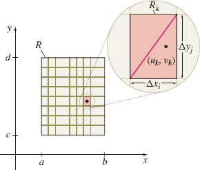
For a function \(f\) of two variables, the double integral of \(f\) is defined similarly. We begin with a function \(z=f(x, y) \) of two variables defined over a closed rectangular region \(R\) defined by \(a\leq x\leq b\) and \(c\leq y\leq d.\) We partition the interval \([ a, b ] \) into \(n\) subintervals of length \(\Delta x_{i}\), \(i=1, 2, \ldots, n\), and partition the interval \([c, d] \) into \(m\) subintervals of length \(\Delta y_{j}\), \(j=1, 2, \ldots, m\).
This partitions the rectangular region \(R\) into \(N=nm\) subrectangles \(R_{k}\), each of area \(\Delta A_{k}=\Delta x_{i}\Delta y_{j},\) and forms a rectangular partition \(P\) of the region \(R.\) We define the norm \( \left\Vert P\right\Vert \) of the partition as the length of the longest diagonal of the subrectangles \(R_{k},\) \(k=1, 2, 3,\ldots ,N\). See Figure 1.
In each subrectangle \(R_{k}\), we choose a point \((u_{k},v_{k})\) and evaluate the function \(z=f(x, y) \) at \((u_{k}, v_{k})\). Then we multiply \(f(u_{k}, v_{k})\) by the area \(\Delta A_{k}=\Delta x_{i} \Delta y_{j}\) of \( R_{k}\), \(k=1, 2, \ldots, N,\) and form the sums \[\bbox[5px, border:1px solid black, #F9F7ED]{ \sum\limits_{k=1}^{N}f(u_{k},v_{k})\Delta A_{k} } \]
These are the Riemann sums of \(f\) for the partition \(P.\)
905
EXAMPLE 1Finding Riemann Sums
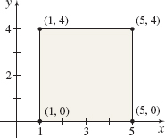
Let \(f(x, y)=x^{2}y\) be a function defined over the square having its lower left corner at \((1, 0)\) and its upper right corner at \((5, 4)\), as shown in Figure 2.
- (a) Find a Riemann sum of \(f\) over this region by partitioning the square into four congruent subsquares. Choose the lower left corner of each subsquare as \((u_{k},v_{k})\), \(k=1, 2, 3, 4.\)
- (b) Find a Riemann sum of \(f\) over the partition used in (a) but choose the upper right corner of each subsquare as \((u_{k},v_{k})\), \(k=1, 2, 3, 4.\)
- (c) Find a Riemann sum of \(f\) over this region by partitioning the square into eight congruent rectangles with sides of length \(\Delta x_{i}=2,\) \(i=1, 2,\) and \(\Delta y_{j}=1,\) \(j=1, 2, 3, 4\). Choose the lower right corner of each rectangle as \((u_{k}, v_{k}) ,\) \(k=1, 2, \ldots, 8.\)
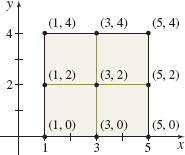
Solution (a) We begin by partitioning the square in Figure 2 into \(N=4\) congruent subsquares, as shown in Figure 3. For each subsquare, \(\Delta A_{k}=(2) (2) =4\). The Riemann sum for which \( (u_{k},v_{k})\) is the lower left corner of each subsquare is \[ \begin{eqnarray*} \sum_{k=1}^{4}f(u_{k},v_{k})\Delta A_{k} &=&f(1, 0)(4) +f(3, 0) (4) +f(1, 2) (4) +f(3, 2) (4) \\[3pt] &=&[f(1, 0)+f(3, 0) +f(1, 2) +f(3, 2)] (4)\\[3pt] &=&(0+0+2+18) (4) =80 \qquad\qquad {\color{#0066A7}{\hbox{\(f(x, y) =x^{2}y\)}}} \end{eqnarray*} \]
(b) See Figure 3. The Riemann sum using the upper right corner of each subsquare for \((u_{k},v_{k})\) is \[ \begin{eqnarray*} \sum_{k=1}^{4}f(u_{k},v_{k})\Delta A_{k}& =&f(3, 2) (4) +f(5, 2) (4) +f(3, 4) (4) +f(5, 4) (4) \\[4pt] &=&[ f(3, 2) +f(5, 2) +f(3, 4)+f(5, 4) ] (4)\\[4pt] &=&(18+50+36+100)(4) =816 \end{eqnarray*} \]
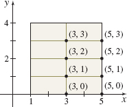
(c) Now we partition the square in Figure 2 into \(N=8\) congruent rectangles with sides \(\Delta x_{i}=2,\) \(i=1, 2,\) and \(\Delta y_{j}=1\), \( j=1, 2, 3, 4,\) as shown in Figure 4. The Riemann sum, for which \((u_{k}, v_{k}),\) \(k=1, 2, 3,\ldots, 8,\) is the lower right corner of each rectangle and \( \Delta A_{k}=(2) (1) =2\), is \[ \begin{eqnarray*} \sum_{k=1}^{8}f(u_{k},v_{k})\Delta A_{k} &=&f(3,0) (2) +f(5,0) (2) +f(3,1) (2) +f(5,1) (2) +f(3,2) (2)\\[4pt] &&+\,f(5,2) (2) +f(3,3) (2) +f(5,3) (2) \\[4pt] &=&[ f(3,0) +f(5,0) +f(3,1) +f(5,1) +f(3,2) +f(5,2)\\[4pt] &&+\,f(3,3) +f(5,3) ] (2) \\[4pt] &=&( 0+0+9+25+18+50+27+75) (2) =408 \end{eqnarray*} \]
NOW WORK
As Example 1 demonstrates, the Riemann sums of a function \(z=f(x, y)\) over a region \(R\) depend on both the choice of the partition, which depends on \(\Delta x_{i}\), \(i=1, 2, \ldots, n\), and \(\Delta y_{j}\), \(j=1, 2, \ldots, m\), and the choice of the points \((u_{k},v_{k})\), \(k=1, 2,\ldots,N\), where \(N=nm\). If \(\lim\limits_{\Vert P\Vert \rightarrow 0}\sum\limits_{k=1}^{N}f(u_{k},v_{k})\Delta A_{k}=I\) exists and does not depend on the choice of the partition or on the choice of (\(u_{k}, v_{k}\)) , then the number \(I\) is called the double integral of \( z=f(x, y) \) over the region \(R\) and is denoted by \(\displaystyle \iint\limits_{\kern-3ptR}f(x, y)\, {\it dA}.\)
906
DEFINITION Double Integral
Let \(f\) be a function of two variables defined on a closed rectangular region \(R\). Then the double integral of \(f\) over \(R\), denoted by \(\displaystyle\iint\limits_{\kern-3ptR}f(x, y)~{\it dA}\), is defined by \[\bbox[5px, border:1px solid black, #F9F7ED]{ \displaystyle\iint\limits_{\kern-3ptR}f(x, y)\, {\it dA}=\lim\limits_{\Vert P\Vert \rightarrow 0}\sum\limits_{k=1}^{N}f(u_{k},v_{k})\Delta A_{k} } \]
provided this limit exists. In this case, \(f\) is said to be integrable on \(R\).
Since \(\Delta x_{i}\Delta y_{j}=\Delta y_{j}\Delta x_{i}=\Delta A_{k},\) other symbols for the double integral of \(f\) over \(R\) are \[ \displaystyle\iint\limits_{\kern-3ptR}f(x, y)\,{\it dx}\,{\it dy}\qquad \hbox{and}\qquad \displaystyle\iint\limits_{\kern-3ptR}f(x, y)\,{\it dy}\,{\it dx} \]
In Chapter 5, an important theorem stated that if a function \(f\) is continuous on a closed interval \([a, b],\) then \( \int_{a}^{b}f(x)\,{\it dx}\) exists. A similar result holds for functions of two variables.
THEOREM Existence of the Double Integral
If a function \(z=f(x, y) \) is continuous on a closed, rectangular region \(R,\) then the double integral \(\displaystyle\iint\limits_{\kern-3ptR}f(x, y)\,{\it dA}\) exists.
A proof can be found in most advanced calculus books.
2 Find the Value of a Double Integral Defined on a Closed Rectangular RegionPrinted Page 906
To find the value of a double integral of a function \(f\) of two variables whose domain is a closed rectangle without using Riemann sums, we need the concept of partial integration. Partial integration is the process of finding the single integral of a function \(f\) of two variables with respect to one variable, while treating the other variable as a constant. The symbol \(\int_{a}^{b}f(x, y)\,{\it dx}\) means treat \(y\) as a constant and integrate \(f\) with respect to the variable \(x\). The result is a function of \(y\) alone. Similarly, \(\int_{c}^{d}f(x, y)\, {\it dy}\) means treat \(x\) as a constant and integrate \(f\) with respect to the variable \(y\). This result is a function of \(x\) alone.
IN WORDS
Partial Integration is the reverse of partial differentiation.
EXAMPLE 2Using Partial Integration
Use partial integration to find:
- (a) \(\int_{1}^{2} x^{3}y^2\,{ dx}\)
- (b) \(\int_{0}^{4}x^{3}y^2\, {dy}\)
Solution (a) For \(\int_{1}^{2} x^{3}y^2\,{\it dx}\), we treat \(y\) as a constant and integrate with respect to \(x\): \[ \int_{1}^{2} x^{3}y^2\,{\it dx}=y^2\int_{1}^{2}x^{3}{\it dx}=y^2\left[ \dfrac{x^{4}}{4}\right] _{1}^{2}= y^2\left( 4-\dfrac{1}{4}\right) =\dfrac{15}{4}y^2 \]
(b) For \(\int_{0}^{4} x^{3}y^2\, {\it dy},\) we treat \(x\) as a constant and integrate with respect to \(y\): \[ \int_{0}^{4} x^{3}y^2\, {\it dy}= x^{3}\!\int_{0}^{4}y^2\, {\it dy}= x^{3}\left[ {\dfrac{y^{3}}{3}} \right] _{0}^{4}=\dfrac{64x^{3}}{3} \]
NOW WORK
907
EXAMPLE 3Using Partial Integration
Use partial integration to find:
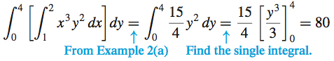
- (a) \(\int_{0}^{4}\left[ \int_{1}^{2} x^{3}y^2\,{dx}\right] \!{\it dy}\)
- (b) \(\int_{1}^{2}\left[ \int_{0}^{4} x^{3}y^2\,{\it dy}\right] \! {dx}\)
Solution (a) We begin by using partial integration to find the integral within the bracket. Then we integrate the result with respect to \( y.\)
(b) 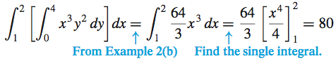
NOW WORK
Integrals of the form \[ \int_{a}^{b}\left[ \int_{c}^{d}f(x, y)\,{\it dy}\right] \! {\it dx}\qquad \hbox{and} \qquad \int_{c}^{d}\left[ \int_{a}^{b}f(x, y)\,{\it dx}\right] \! {\it dy} \]
are called iterated integrals. In the iterated integral on the left, we integrate the function \(f\) partially with respect to \(y\) from \(c\) to \(d,\) obtaining a function of \(x\) that we then integrate with respect to \( x\) from \(a\) to \(b\). In the iterated integral on the right, we integrate \(f\) partially with respect to \(x\) from \(a\) to \(b,\) obtaining a function of \(y\) that we then integrate with respect to \(y\) from \(c\) to \(d\).
Notice in Example 3 that the iterated integrals \(\int_{0}^{4}\big[ \int_{1}^{2}x^{3}y^{2}\, { dx} \big] { dy}\) and \(\int_{1}^{2} \big[\int_{0}^{4}x^{3}y^{2}\,{ dy}\big] { dx}\) are equal. This is a consequence of Fubini’s Theorem, which provides a practical way to find certain double integrals.
ORIGINS
Guido Fubini (1879–1943) was an Italian mathematician born in Venice. His father was a mathematics teacher who encouraged Guido to study mathematics. A short man, Fubini made many contributions in diverse areas of math, earning him the nickname “the little giant.” In 1939 the anti-Semitic policies of Mussolini caused Fubini and his family to immigrate to the United States. He accepted a position at the Institute for Advanced Study in Princeton, NJ, and also taught at Princeton University for several years. He died in New York in 1943.
THEOREM Fubini's Theorem
If a function \(z=f(x, y)\) is continuous on a closed rectangular region \(R\) defined by \(a\leq x\leq b\) and \(c\leq y\leq d\), then \[\bbox[5px, border:1px solid black, #F9F7ED]{ \displaystyle\iint\limits_{\kern-3ptR}f(x, y)\,{dA}=\int_{a}^{b}\left[ \int_{c}^{d}f(x, y)\,{dy}\right] \! {dx}=\int_{c}^{d}\left[ \int_{a}^{b}f(x, y)\,{dx} \right]\! {dy} } \]
Fubini's Theorem states that an iterated integral can be integrated in either order provided the function \(z=\) \(f(x, y) \) is continuous on the closed rectangular region \(R\).
EXAMPLE 4Finding the Value of a Double Integral Using Fubini’s Theorem
Find the value of \(\displaystyle\iint\limits_{\kern-3ptR}(2x+y)\,{\it dA}\) if \(R\) is the closed rectangular region defined by \(1\leq x\leq 5\) and \(0\leq y\leq 4\).
Solution Using Fubini’s Theorem, the double integral \(\iint\limits_{\kern-3ptR}(2x+y)\,{\it dA}\) equals either of the iterated integrals \[ \begin{equation} \displaystyle\int_{1}^{5}\left[ \int_{0}^{4}(2x+y)\,{dy}\right]\! {dx}\qquad \hbox{or} \qquad \displaystyle\int_{0}^{4} \left[ \int_{1}^{5}(2x+y)\,{dx}\right]\! {dy} \tag{1} \end{equation} \]
908
Below we find the integral on the left. \[ \begin{eqnarray*} \displaystyle\iint\limits_{\kern-3ptR}(2x+y)\,{\it dA}&=&\int_{1}^{5}\left[ \int_{0}^{4}(2x+y)\,{\it dy}\right]\! {\it dx} \underset{\underset{\underset{{\color{#0066A7}{\hbox{with respect to $y$}}}}{\color{#0066A7}{\hbox{Integrate partially }}}}{\color{#0066A7}{\uparrow }}}{=}\int_{1}^{5} \left[2xy + \dfrac{y^{2}}{2}\right] _{0}^{4}\,{\it dx} \\ &=& \int^5_1 (8x+8)\,{\it dx} = \big[4x^2+8x\big]^5_1 = 140-12=128 \end{eqnarray*} \]
NOW WORK
Example 4 using the integral on the right in (1).
NOW WORK
3 Find the Volume Under a Surface and over a Rectangular RegionPrinted Page 908
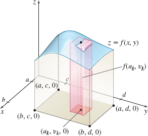
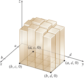
The double integral \(\displaystyle\iint\limits_{\kern-3ptR}f(x,y)\,{\it dA}\) over a rectangular region \( R \) has a geometric interpretation. If the function \(z=f(x,y) \) is nonnegative over \(R\), then \(f(u_{k},v_{k}) \) represents the height of \(z\) at the point \((u_{k},v_{k}) ,\) and the product \( f(u_{k},v_{k}) \Delta A_{k}\) can be thought of as the volume of a small, rectangular cylinder of height \(f(u_{k},v_{k}) \) with a base of area \(\Delta A_{k}\), as shown in Figure 5. The sum of the volumes of these small cylinders, \(\sum\limits_{k=1}^{N}f(u_{k},v_{k}) \Delta A_{k}\), is an approximation for the volume of the solid under the graph of \(z=f(x,y) \), and over \(R\) as illustrated in Figure 6. If \(f\) is continuous over \(R\), then \(\lim\limits_{\Vert P\Vert \rightarrow 0}\sum\limits_{k=1}^{N}f(u_{k},v_{k}) \Delta A_{k}\) exists, and \(\displaystyle\iint\limits_{\kern-3ptR}f(x,y)\, {\it dA}\) can be interpreted as the volume of the solid under the graph of \(z=f(x,y) \) and over the region \(R\).


NOTE
It can be proved that this formula for volume is consistent with the formulas for volume given in Chapter 6.
Volume Under a Surface
Let \(z=f(x,y) \) be a function of two variables that is continuous and nonnegative on a closed, rectangular region \(R\). The volume \( V \) under the surface \(z=f(x,y)\) and over the region \(R\) is given by \[\bbox[5px, border:1px solid black, #F9F7ED]{ V=\displaystyle\iint\limits_{\kern-3ptR}f(x,y)\,{\it dA} } \]
909
EXAMPLE 5Finding the Volume of a Solid
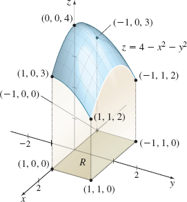
Find the volume \(V\) under the paraboloid \(z=f(x,y)=4-x^{2}-y^{2}\) and over the rectangular region \(R\) defined by \(-1\leq x\leq 1\) and \(0\leq y\leq 1\).
Solution We begin by graphing \(z=f(x,y) \) and the rectangular region \(R\), as shown in Figure 7.
Since \(z=f(x,y)\) is continuous and \(z\geq 0\) over the rectangular region \(-1\leq x\leq 1,\) \(0\leq y\leq 1\) , the volume \(V\) under the surface \(z=f(x,y) \) is given by \[ V=\displaystyle\iint\limits_{\kern-3ptR}f(x,y)\,{\it dA}=\displaystyle\iint\limits_{\kern-3ptR}(4-x^{2}-y^{2})\,{\it dA} \]
Using Fubini’s Theorem, we have \begin{eqnarray*} V& =&\int_{-1}^{1}\left[ \int_{0}^{1}(4-x^{2}-y^{2})\,{\it dy}\right]\! {\it dx}=\int_{-1}^{1}\left[ 4y-x^{2}y-\dfrac{y^{3}}{3}\right]_{0}^{1}\,{\it dx}\\[4pt] &=&\int_{-1}^{1}\left( 4-x^{2}-\dfrac{1}{3}\right)\!{\it dx}=\int_{-1}^{1}\left( \dfrac{11}{3}-x^{2}\right)\!{\it dx}=\left[ \dfrac{11}{3}x-\dfrac{x^{3}}{3}\right] _{-1}^{1}\\[4pt] &=&\left( \dfrac{11}{3}-\dfrac{1}{3}\right) -\left( -\dfrac{11}{3}+\dfrac{1}{3}\right) =\dfrac{20}{3}\hbox{ cubic units} \end{eqnarray*}
NOW WORK
Example 5 by finding \(\int_{0}^{1}\left[ \int_{-1}^{1}(4-x^{2}-y^{2})\,{\it dx}\right] \! {\it dy}.\)