11 Categorical Data Analysis

11.1 $χ^{2}$ Goodness of Fit Test

This page includes Video Technology Manuals

OBJECTIVES By the end of this section, I will be able to …

Explain what a multinomial random variable is and how to calculate expected frequencies.
Describe how a $χ^{2}$ goodness of fit test works.
Perform and interpret the results from the $χ^{2}$ goodness of fit test using the critical-value method and the p-value method.

According to the Adobe Digital Index, the market share for the leading Internet browsers (both desktop and mobile) in June 2014 was as follows: Google Chrome, 32%; Microsoft Internet Explorer, 31%; others, 37%. Change is rapid in the online environment. Have these market shares changed since June 2014? How would we go about performing a hypothesis test to determine whether market shares have changed significantly? In Section 11.1, we examine this question using a new type of hypothesis test called a $χ^{2}$ goodness of fit test. We begin by first considering a new type of random variable that is used to represent categorical data.

1 The Multinomial Random Variable

Recall from Chapter 1 that categorical (qualitative) variables take values that can be classified into categories. In Chapter 6, we considered binomial random variables, for which there are only two possible outcomes. Now, let's consider the following type of random variable, which can have more than two possible values.

Multinomial Random Variable

A random variable is multinomial if it satisfies each of the following conditions:

Each independent trial of the experiment has $k$ possible outcomes, $k = 2, 3, 4, \dots$
The ith outcome (category) occurs with probability $p_{i}$ , where $i = 1, 2, \dots, k$ (that is, $p_{i}$ is the population proportion for category $i$ ).
$\sum p_{i} = 1$ (Law of Total Probability).

Data from a multinomial random variable are said to follow a multinomial distribution.

Note: The binomial distribution may be considered a special case of the multinomial distribution, with $k = 2$ .

For example, suppose 30% of the residents of a particular town are Democrats,30% are Republicans, and 40% are Independents. If we select $n = 100$ residents at random, then the number of Democrats, Republicans, and Independents observed follows a multinomial distribution, with

$P_{Democrats} = 0.30, P_{Republicans} = 0.30, P_{Independents} = 0.40,$

and

$\sum p_{i} = 0.30 + 0.30 + 0.40 = 1$

EXAMPLE 1 Identifying a Multinomial Random Variable

For each of the following, determine whether the random variable is multinomial.

We select 10 students at random and define our random variable $X$ to be the amount of time the student used a Web browser yesterday.
We select 10 students at random and define our random variable $X$ to be the browser used most by the student the last time he or she was on the Internet, where the possible values are Google Chrome, Microsoft Internet Explorer, or Other.

Page 633

Solution

The amount of time spent using a browser is a continuous random variable, not categorical. So, $X$ cannot be multinomial.
The browser is categorical. We have $k = 3$ different categories, with the population proportions of the three categories adding up to one (see Example 2(a) below). Therefore, $X$ is multinomial.

NOW YOU CAN DO

Exercises 5–8

Next, recall from Section 6.2 that the formula for finding the expected value (mean) of a binomial random variable having $n$ trials and probability of success $p$ is

$expected value = n \cdot p$

For a multinomial random variable, the expected frequency of the ith category is

${expected frequency}_{i} = E_{i} = n \cdot p_{i}$

where $n$ represents the number of trials, and $p_{i}$ represents the population proportion for the ith category.

EXAMPLE 2 Finding the expected frequencies

According to the Adobe Digital Index, the market share for the leading Internet browsers (both desktop and mobile) in June 2014 was as shown in Table 1. Let $X = b r o w s e r$ of a randomly selected Internet user.

Verify that $X = b r o w s e r$ is a valid multinomial random variable.
Find the expected frequency for each category in a series of 200 trials.

Table 11.1: Table 1 Distribution of browser market share

Browser	Relative frequency
Google Chrome	0.32
Microsoft Internet Explorer	0.31
Other	0.37

Solution

There are $k = 3$ possible outcomes: Google Chrome, Microsoft Internet Explorer, and Other. Assigning probabilities using the relative frequency method, we have the following hypothesized proportions for each browser:

$p_{Chrome} = 0.32, p_{IE} = 0.31, p_{Other} = 0.37$

and

$\sum p_{i} = 0.32 + 0.31 + 0.37 = 1$

Therefore, $X = b r o w s e r$ is a valid multinomial random variable.

Page 634
We have $n = 200$ trials ( $sample size = 200$ ), so the expected frequencies are as provided in Table 2.

Table 11.2: Table 2 Expected frequencies for browser preference in sample of size 100

Category	$E x p e c t e d f r e q u e n c y_{i} = E_{i} = n \cdot p_{i}$
Google Chrome	$E_{Chrome} = 200 \cdot 0.32 = 64$
Microsoft Internet Explorer (IE)	$E_{IE} = 200 \cdot 0.31 = 62$
Other	$E_{Others} = 200 \cdot 0.37 = 74$

As a check on the calculations, we should have $\sum E_{i} = n$ . In this case,

$\sum E_{i} = 64 + 62 + 74 = 200 = n$

NOW YOU CAN DO

Exercises 9–12.

YOUR TURN#1

Verify that $X = b o o k f o r m a t$ is a valid multinomial random variable.
Find the expected frequency for each category.

(The solutions are shown in Appendix A.)

What Do These Expected Frequencies Mean?

Recall that the expected value of a random variable refers to the long-run mean of that random variable after an arbitrarily large number of trials. For example, if we repeatedly took samples of 200 Internet users and asked about browser preference, the mean number of persons who used Google Chrome would approach $E_{Chrome} = 64$ as we took more and more different samples, if the proportions given in Table 1 are correct. Similarly, because 31% of the entire population of Internet users use Microsoft IE, we would expect about 31% of any given sample of 200 Internet users to use Microsoft IE, because the sample is a subset of the population. This of course raises the question: Are the proportions in Table 1 still true? That is the type of question we will learn how to address next.

2 What Is a $χ^{2}$ Goodness of Fit Test?

Do the 2014 market shares still hold true today? In other words, has the distribution of the multinomial random variable browser given in Table 1 changed since June 2014? To determine this, we introduce a new type of hypothesis test, called a $χ^{2}$ goodness of fit test.

$χ^{2}$ Goodness of Fit Test

A $χ^{2}$ goodness of fit test is a hypothesis test used to determine whether a random variable follows a particular distribution. In a goodness of fit test, the hypotheses are

$H_{0} : The random variable follows a purticular distribution$
$H_{a} : The random variable does not follow the distribution specified in H_{0}$ .

Page 635

For Example 2, the null hypothesis completely specifies each of the probabilities in the relative frequency distribution, as follows:

$H_{0} : p_{Chrome} = 0.32, P_{IE} = 0.31, p_{Other} = 0.37$

The alternative hypothesis simply denies the claim made by the null hypothesis:

$H_{a} : The random variable does not follow the distribution specified in H_{0}$ .

In other words, $H_{a}$ claims that the browser market shares have changed since June 2014.

Developing Your Statistical Sense

Fitting the Model to the Data

Now, a goodness of fit test sounds like something you do in a clothing store dressing room. Actually, the analogy to clothes is rather appropriate. Suppose winter is coming and you are in the market for a new pair of gloves. You find one pair that is especially attractive, but the gloves don't fit your hands. What do you do? You reject the ill-fitting gloves and search for a new pair. In statistics, the gloves represent the models and your hands represent the actual “hard data” observed in the sample.

The null hypothesis $H_{0}$ represents what is called a model, a working theory of how the population proportions are distributed. Our working model of how the market shares are distributed is stated in the null hypothesis:

Model 1. $H_{0} : p_{Chrome} = 0.32, p_{IE} = 0.31, p_{Other} = 0.37$

Of course, we could also try other models if we think the market has changed, such as the following:

Model 2. $H_{0} : p_{Chrome} = 0.33, p_{IE} = 0.33, p_{Other} = 0.34$

Model 3. $H_{0} : p_{Chrome} = 0.40, p_{IE} = 0.30, p_{Other} = 0.30$

In hypothesis testing, we “try on” only one model at a time.

In statistics, a goodness of fit test determines if the actual “hard data” observed in the sample are consistent with the proportions stated in the null hypothesis. Market researchers would collect data on the actual preferences of a sample of 100 real Internet users in order to determine whether or not the market shares have changed. The sample is summarized in a set of observed frequencies of Internet users who prefer the various browsers. The $χ^{2}$ goodness of fit test then compares these observed frequencies with the expected frequencies found in Example 2.

How a Goodness of Fit Test Works

The goodness of fit test is based on a comparison of the observed frequencies (sample data) with the expected frequencies when $H_{0}$ is true. That is, we compare what we actually see with what we would expect to see if $H_{0}$ were true. If the difference between the observed and expected frequencies is large, we reject $H_{0}$ .

The difference between the observed and expected frequencies is measured by the test statistic, $χ_{data}^{2}$ . As usual, it comes down to how large a difference is large.

Page 636

Test Statistic for the $χ^{2}$ Goodness of Fit Test

For a multinomial random variable with $k$ categories and $n$ trials, let $O_{i}$ represent the observed frequency for category $i$ , and let $E_{i}$ represent the expected frequency for category $i$ . Then the test statistic for a goodness of fit test

$χ_{data}^{2} = \sum \frac{{(O_{i} - E_{i})}^{2}}{E_{i}}$

approximately follows a $χ^{2}$ (chi-square) distribution with $k - 1$ degrees of freedom (df), if the following conditions are satisfied:

None of the expected frequencies is less than 1.
At most, 20% of the expected frequencies are less than 5.

Students may want to review the characteristics of the $χ^{2}$ distribution (Chapter 10, page 618) and the procedure for finding $χ^{2}$ critical values for a right-tailed test (Chapter 10, page 620).

If the conditions are not satisfied, then it may be possible to combine two or more categories so that the conditions may then be fulfilled.

EXAMPLE 3 Calculating $χ_{data}^{2}$

Suppose the observed frequencies of browser preference in Table 3 come from a survey taken this year of 200 Internet users.

Table 11.3: Table 3 Observed frequencies of browser preference in a sample of 200 Internet users

Browser	Observed frequency
Google Chrome	80
Microsoft Internet Explorer	62
Other	58

Calculate the test statistic $χ_{data}^{2}$ by comparing the observed frequencies from Table 3 with the expected frequencies calculated in Table 2 of Example 2.

Solution

The observed frequencies $O_{i}$ are found in Table 3, and the expected frequencies are given in Table 2. Table 4 then provides the quantities needed to calculate $χ_{data}^{2}$ . Then

$χ_{data}^{2} = \sum \frac{{(O_{i} - E_{i})}^{2}}{E_{i}} \approx 4 + 0 + 3.46 = 7.46$

Table 11.4: Table 4 Calculating

$χ_{data}^{2}$

Category	$p_{i}$	$O_{i}$	$E_{i}$	$O_{i} - E_{i}$	${(O_{i} - E_{i})}^{2}$	$\frac{{(O_{i} - E_{i})}^{2}}{E_{i}}$
Chrome	0.32	80	64	16	256	$\frac{{(80 - 64)}^{2}}{64} = 4$
IE	0.31	62	62	0	0	$\frac{{(62 - 62)}^{2}}{62} = 0$
Other	0.37	58	74	−16	−256	$\frac{{(58 - 74)}^{2}}{74} \approx 3.46$

NOW YOU CAN DO

Exercises 13–18.

Page 637

YOUR TURN#2

Publishers Weekly reported that, in 2014, the book format market share was as follows: paperbacks, 41%; hard covers, 34%; e-books, 13%; and all other formats, 12%. Suppose a survey was conducted this year of 2000 books purchased, with the following book sales: 810 paperbacks, 680 hard covers, 280 e-books, and 230 others. Calculate the test statistic $χ_{data}^{2}$ .

(The solution is shown in Appendix A.)

3 Performing the $χ^{2}$ Goodness of Fit Test

The $χ^{2}$ goodness of fit test may be performed using (a) the critical-value method or (b) the p-value method. We start with the critical value method.

$χ^{2}$ Goodness of Fit Test: Critical-Value Method

Step 1 State the hypotheses and check the conditions.

The null hypothesis states that the multinomial random variable follows a particular distribution.
The alternative hypothesis states that the random variable does not follow that distribution.

The following conditions must be met:

None of the expected frequencies is less than 1.
At most, 20% of the expected frequencies are less than 5.

The expected frequency for the ith category is $E_{i} = n \cdot p_{i}$ , where $n$ represents the number of trials and $p_{i}$ represents the population proportion for the ith category.

Step 2 Find the $χ^{2}$ critical value, $χ_{crit}^{2}$ , and state the rejection rule. Use Table E in the Appendix. Reject $H_{0} if χ_{data}^{2} \geq χ_{crit}^{2}$
Step 3 Calculate $χ_{data}^{2}$ .

$χ_{data}^{2} = \sum \frac{{(O_{i} - E_{i})}^{2}}{E_{i}}$

where $O_{i}$ = observed frequency, and $E_{i}$ = expected frequency.
Step 4 State the conclusion and the interpretation. Compare $χ_{data}^{2} with χ_{crit}^{2}$ .

All hypothesis tests in this chapter are right-tailed tests, so that we need to find $χ_{crit}^{2}$ for the area to the right of the critical value only.

EXAMPLE 4 Critical-value method for the $χ^{2}$ goodness of fit test

Test whether the Internet browser market shares from Example 2 have changed since June 2014, using level of significance $α = 0.05$ .

Solution

Step 1 State the hypotheses and check the conditions. The hypotheses are:

$\begin{array}{l} H_{0} : p_{Chrome} = 0.32, p_{IE} = 0.31, p_{Other} = 0.37 \\ H_{a} : The random variable does not follow the distribution specified in H_{o.} \end{array}$

Checking the conditions, the expected frequencies from Table 2 are

$E_{Chrome} = 64, E_{IE} = 62, E_{Other} = 74$

Because none of these expected frequencies is less than 1, and none of the expected frequencies is less than 5, the conditions for performing the goodness of fit test are satisfied.
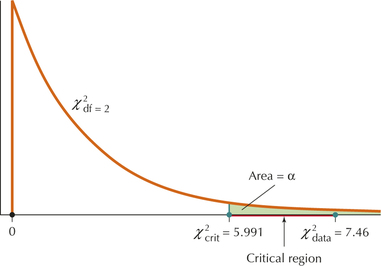
Step 2 Find the $χ^{2}$ critical value, $χ_{crit}^{2}$ , and state the rejection rule. We have degrees of freedom $k - 1 = 3 - 1 = 2 and α = 0.05.$ . Turning to the $χ^{2}$ table (Table E in the Appendix) in the column labeled $χ_{0.05}^{2}$ and the row containing $df = 2$ , we find $χ_{crit}^{2} = χ_{0.05}^{2} = 5.991$ , as shown in Figure 1. The rejection rule is “Reject $H_{0}$ if $χ_{data}^{2} \geq 5.991$ ."

Page 638

FIGURE 1 Finding the $χ^{2}$ critical value for $df = k - 1 = 2$ and level of significance $α = 0.05$ .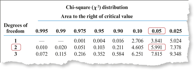
Step 3 From Example 3, we have $χ_{data}^{2} = 7.46$ .
Step 4 State the conclusion and the interpretation. Compare $χ_{data}^{2} with χ_{crit}^{2} . χ_{data}^{2} = 7.46$ is greater than $χ_{crit}^{2} = 5.991$ , as shown in Figure 2. Therefore, we reject $H_{0}$ .

FIGURE 2 Reject $H_{0}$ when $χ_{data}^{2} \geq χ_{crit}^{2} .$

Evidence exists at level of significance $α = 0.05$ that the random variable browser does not follow the distribution specified in $H_{0}$ . In other words, evidence exists that the market shares for Internet browsers have changed.

NOW YOU CAN DO

Exercises 19–22.

YOUR TURN#3

Test using level of significance $α = 0.05$ whether the book format market shares have changed, using the information from Your Turn #1 on page 634 and Your Turn #2 on page 637.

(The solution is shown in Appendix A.)

Developing Your Statistical Sense

Be Careful How You Interpret the Conclusion

Note carefully what this conclusion says and what it doesn't say. The $χ^{2}$ goodness of fit test provides evidence that the random variable does not follow the distribution specified in $H_{0}$ . In particular, the conclusion does not state, for example, that Chrome's proportion is significantly greater than it was in 2014. Informally, we can compare the observed frequency of 80 with the expected frequency of 64 for the Chrome browser and note that there appears to be evidence of an increase in market share for Chrome. But this is only informal and is not part of the hypothesis test. It is a common error in statistical analysis to form conclusions beyond what the hypothesis test is actually testing.

Page 639

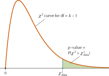
Next, we turn to the p-value method. The $χ^{2}$ goodness of fit test is a right-tailed test, so the p-value for the $χ^{2}$ statistic is defined as the area under the $χ^{2}$ curve to the right of the test statistic $χ_{data}^{2}$ , as shown in Figure 3. That is,

$p -value = P (χ^{2} > χ_{data}^{2})$

FIGURE 3

$p -Value = P (χ^{2} > χ_{data}^{2}) .$

$χ^{2}$ Goodness of Fit Test: p-Value Method

Step 1 State the hypotheses and the rejection rule. Check the conditions.

The null hypothesis states that the multinomial random variable follows a particular distribution.
The alternative hypothesis states that the random variable does not follow that distribution.
Reject $H_{0}$ if the p-value $\leq α$ .

The following conditions must be met:

None of the expected frequencies is less than 1.
At most, 20% of the expected frequencies are less than 5.

The expected frequency for the ith category is $E_{i} = n \cdot p_{i}$ , where $n$ represents the number of trials and $p_{i}$ represents the population proportion for the ith category.

Step 2 Calculate $χ_{data}^{2}$ .

$χ_{data}^{2} = \sum \frac{{(O_{i} - E_{i})}^{2}}{E_{i}}$

where $O_{i}$ = observed frequency, and $E_{i}$ = expected frequency.
Step 3 Find the p-value.

$p -value = P (χ^{2} > χ_{data}^{2})$ (see Figure 3)
Step 4 State the conclusion and the interpretation. Compare the p-value with $α$ .

EXAMPLE 5 p-Value method for the $χ^{2}$ goodness of fit test using technology

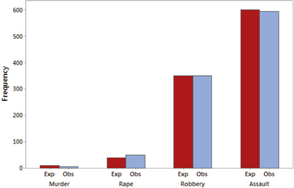
Table 5 contains the distribution of violent crime in New York City in 2012.² Suppose that a random sample of 1000 violent crimes in New York City yielded the counts shown in Table 6. Test whether the population proportions have changed since 2012, using the p-value method and level of significance $α = 0.05$ .

Table 11.5: Table 5 2012 violent crime in New York City

Murder	Rape	Robbery	Assault
0.01	0.04	0.35	0.60

Page 640

Table 11.6: Table 6 Sample of 1000 violent crimes in New York City this year

Murder	Rape	Robbery	Assault
6	50	350	594

Solution

Step 1 State the hypotheses and the rejection rule. Check the conditions.
$\begin{array}{l} H_{0} : p_{Murder} = 0.01, p_{Rape} = 0.04, p_{Robbery} = 0.35, p_{Assault} = 0.60 \\ H_{a} : The random variable does not follow the distribution specified in H_{0} \end{array}$

Reject $H_{0}$ if the p-value $\leq 0.05$ .

What Results Might We Expect?

Before we do the formal hypothesis test, let's try to figure out what the conclusion might be. Figure 4 is a clustered bar graph (see Section 2.1) of the observed and expected frequencies for each of the four categories. If $H_{0}$ were true, then, for each category, we would expect the red bars (observed frequencies) and blue bars (expected frequencies) to have somewhat similar heights. In fact, the heights of the bars are fairly similar for all four categories, indicating not much difference between the crimes that were observed and the crimes that were expected. Thus, we might expect to not reject $H_{0}$ .

FIGURE 4 Graph indicates no evidence against

$H_{0}$ .

First, we need to find the expected frequencies. We have $n = 1000$ , so the expected frequencies are as shown here.

Category	$E x p e c t e d f r e q u e n c y_{i} = E_{i} = n \cdot p_{i}$
Murder	$E_{Murder} = 1000 \cdot 0.01 = 10$
Rape	$E_{Rape} = 1000 \cdot 0.04 = 40$
Robbery	$E_{Robbery} = 1000 \cdot 0.35 = 350$
Assault	$E_{Assault} = 1000 \cdot 0.60 = 600$

Table 11.7: Expected frequencies for violent crimes in a sample of size

$n = 1000$

Page 641

Next, check the conditions for this test. Because (a) none of the expected frequencies is less than 1 and (b) no more than 20% of the expected frequencies are less than 5, we may proceed. We use the instructions provided in the Step-by-Step Technology Guide at the end of this section.

Step 2 Find the test statistic $χ_{data}^{2}$ . The TI-83/84 results in Figure 5 tell us that

$χ_{data}^{2} = 4.16$
Step 3 Find the p-value. Figure 5 also tells us that

$p -value = P (χ^{2} > 4.16) = 0.2446972817 \approx 0.2447$

This p-value, for the χ² distribution with 3 degrees of freedom, is shown in Figure 6.

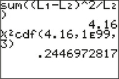FIGURE 5 $χ_{data}^{2} = 4.16$ has p-value 0.2447.

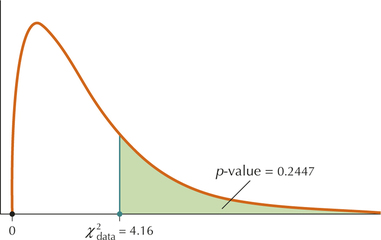FIGURE 6

Figure 7a shows the TI-84 output for the test, and Figure 7b shows the SPSS output for the test, confirming our test statistic of 4.16 and p-value of 0.2447.

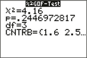FIGURE 7a $χ^{2}$ test on TI-84.

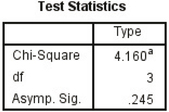FIGURE 7b $χ^{2}$ test in SPSS.
Step 4 State the conclusion and the interpretation. The p-value is not less than $α = 0.05$ , so we do not reject $H_{0}$ , which we expected. There is insufficient evidence, at a level of significance $α = 0.05$ , that the population proportions of violent crime have changed in New York City since 2012.

NOW YOU CAN DO

Exercises 23–26.

11.1 χ2<math><mrow><msup><mi>χ</mi><mn>2</mn></msup></mrow></math> Goodness of Fit Test

11.1 $χ^{2}$ Goodness of Fit Test