11 Categorical Data Analysis

11.2 $χ^{2}$ Tests for Independence and for Homogeneity of Proportions

OBJECTIVES By the end of this section, I will be able to …

Explain what a $χ^{2}$ test for the independence of two variables is.
Perform and interpret a $χ^{2}$ test for the independence of two variables using the critical-value method and the p-value method.
Perform and interpret a test for the homogeneity of proportions.

1 Introduction to the $χ^{2}$ Test for Independence

In Section 11.1, we learned that the $χ^{2}$ distribution could help us determine a model's goodness of fit to the data. Here, in Section 11.2, we will learn two more hypothesis tests that use the $χ^{2}$ distribution. Recall from Section 2.1 that a contingency table, also known as a crosstabulation or a two-way table, is a tabular summary of the relationship between two categorical variables. The categories of one variable label the rows, and the categories of the other variable label the columns. Each cell in the table contains the number of observations that fit the categories of that row and column. Table 7 is a contingency table based on the study How Young People View Their Lives, Futures, and Politics: A Portrait of “Generation Next.”⁵ The researchers asked 1500 randomly selected respondents, “How are things in your life?” Subjects were categorized by age and response. The researchers identified those ages 18–25 as representing “Generation Next.”

The term contingency table derives from the fact that the table covers all possible combinations of the values for the two variables, that is, all possible contingencies.

Table 11.22: Table 7 Contingency table showing relative frequencies of variable categories

	Age group
Response	Gen Nexter (18–25)	26+	Total	Relative frequency
Very happy	180	330	510	$\frac{510}{1500} = 0.34$
Pretty happy	378	435	813	$\frac{813}{1500} = 0.542$
Not too happy	42	135	177	$\frac{177}{1500} = 0.118$
Total	600	900	1500
Relative frequency	$\frac{600}{1500} = 0.4$	$\frac{900}{1500} = 0.6$

We can use contingency tables like Table 7 to determine whether two random variables are independent. Recall that two random variables are independent if the value of one variable does not affect the probabilities of the values of the other variable. For example, is a “Gen Nexter” (someone age 18–25) less likely to report that he or she is “very happy” and more likely to report that he or she is “pretty happy” than someone older? If so, then the response depends on age, so the variables age group and response are dependent.

By “dependent” we simply mean that the variables are not independent.

To determine whether two categorical variables are independent, using the data in a contingency table, we use a $χ^{2}$ test for independence. Just like our $χ^{2}$ goodness of fit test from Section 11.1, the $χ^{2}$ test for independence is based on a comparison of the observed frequencies with the frequencies that are expected if the null hypothesis is assumed true.

Page 647

$χ^{2}$ Test for Independence

To determine whether two categorical variables are independent, using the data from a contingency table, we use a $χ^{2}$ test for independence. The hypotheses take the form

$H_{0} : Variable A and Variable B are independent$ .
$H_{a} : Variable A and Variable B are dependent$ .

We compare the observed frequencies with the frequencies that we expect if we assume that $H_{0}$ is correct. Large differences lead to the rejection of the null hypothesis.

Here, we are testing whether the variables age group and response are independent. Thus, the hypotheses are

$H_{0} : Variable Age group and response are independent$ .
$H_{a} : Variable Age group and response are dependent.$ .

$H_{0}$ states that a response to the survey question does not depend on the age group.

$H_{a}$ says that a response does depend on the age group. To calculate the expected frequencies, we begin by recalling the Multiplication Rule for Two Independent Events from Chapter 5 (page 277):

If $A$ and $B$ are any two independent events, $P (A and B) = P (A) P (B)$ .

To illustrate, let our events be defined as $A = age 18–25 group$ , and $B = reported “very happy.“$ Then, on the assumption that these events are independent, we have

$\begin{array}{l} P (Gen Nexter and very happy) & = & P (A and B) = P (A) P (B) = \frac{600}{1500} \cdot \frac{510}{1500} \\ = & 0.4 \cdot 0.34 = 0.136 \end{array}$

Thus, the probability that a randomly chosen young person is both a Gen Nexter and is very happy is 0.136. Then, to find the expected frequency of this cell (Gen Nexters who are very happy), we multiply this probability 0.136 by the total sample size $n = 1500$ , using the result from Section 11.1 that the expected frequency is

$E = expected frequency = n \cdot p = 1500 \cdot 0.136 = 204$

In other words, if the random variables age group and response are independent, then the expected frequency of Gen Nexters who report being very happy is

$expected {frequency}_{Gen Nexter and very happy} = 1500 \cdot \frac{600}{1500} \cdot \frac{510}{1500} = 204$

But note that two of the 1500s cancel, providing us with the shortcut

$expected {frequency}_{Gen Nexter and very happy} = \frac{(600) (510)}{1500} = 204$

Generalizing, this provides us with the following shortcut method for finding expected frequencies.

Expected Frequencies for a $χ^{2}$ Test for Independence

The expected frequencies for the cells of a contingency table in a $χ^{2}$ test for independence are given by

$expected frequency = \frac{(row total) (column total)}{grand total}$

Page 648

EXAMPLE 6 Calculating expected frequencies using the shortcut method

Calculate the expected frequencies from Table 7 using the shortcut method.

Solution

Table 8 contains the expected frequencies calculated using the shortcut method.

Table 11.23: Table 8 Expected frequencies using the shortcut method

	Age group
Response	Gen Nexter (18–25)	26+	Total
Very happy	$\frac{(510) (600)}{1500} = 204$	$\frac{(510) (900)}{1500} = 306$	510
Pretty happy	$\frac{(813) (600)}{1500} = 325.2$	$\frac{(813) (900)}{1500} = 487.8$	813
Not too happy	$\frac{(177) (600)}{1500} = 70.8$	$\frac{(177) (900)}{1500} = 106.2$	177
Total	600	900	1500

NOW YOU CAN DO

Exercises 5–10.

The $χ^{2}$ test for independence measures the difference between the observed frequencies and the expected frequencies, using the following test statistic.

Test Statistic for the $χ^{2}$ Test for Independence

Let $O_{i}$ represent the observed frequency in the ith cell, and $E_{i}$ represent the expected frequency in the ith cell. Then the test statistic for the independence of two categorical variables

$χ_{data}^{2} = \sum \frac{{(O_{i} - E_{i})}^{2}}{E_{i}}$

approximately follows a $χ^{2}$ distribution with $(r - 1) (c - 1)$ degrees of freedom, where $r$ is the number of categories in the row variable and $c$ is the number of categories in the column variable, if the following conditions are satisfied:

None of the expected frequencies is less than 1.
At most, 20% of the expected frequencies are less than 5.

2 Performing the $χ^{2}$ Test for Independence

The $χ^{2}$ test for independence may be performed using either the critical-value method or the p-value method. We provide examples of each.

$χ^{2}$ Test for Independence: Critical-Value Method

Step 1 State the hypotheses and check the conditions.
- $H_{0} : Variable A and Variable B are independent$ .
- $H_{a} : Variable A and Variable B are dependent.$ .

The following conditions must be met:

None of the expected frequencies is less than 1.
At most, 20% of the expected frequencies are less than 5.

Page 649

The expected frequency for a given cell is

$expected frequency = \frac{(row total) \cdot (column total)}{grand total}$

Step 2 Find the critical value $χ_{crit}^{2}$ and state the rejection rule. Reject $H_{0} if χ_{data}^{2} \geq χ_{crit}^{2} .$ Use $(r - 1) (c - 1)$ degrees of freedom, where r is the number of categories in the row variable and $c$ is the number of categories in the column variable.
Step 3 Calculate $χ_{data}^{2}$ .

$χ_{data}^{2} = \sum \frac{{(O_{i} - E_{i})}^{2}}{E_{i}}$

where $O_{i} = observed frequency$ and $E_{i} = expected frequency for each cell$ .
Step 4 State the conclusion and the interpretation. Compare $χ_{data}^{2} with χ_{crit}^{2} .$

Do not include the row or column totals when counting the categories.

EXAMPLE 7 Performing the $χ^{2}$ test for independence using the critical-value method

Using Table 7, test whether age group is independent of response, using level of significance $α = 0.05$ .

Solution

Step 1 State the hypotheses and check the conditions.
- $H_{0} : Variable Age group and response are independent$ .
- $H_{a} : Variable Age group and response are dependent$ .
We note from Table 8 that none of the expected frequencies are less than either 1 or 5. Therefore, the conditions are met, and we may proceed with the hypothesis test.
See Figure 1 (page 638) to review how to find $χ_{crit}^{2}$ .

Step 2 Find the critical value $χ_{crit}^{2}$ and state the rejection rule. The row variable, response, has three categories, so $r = 3$ . The column variable, age group, has two categories, so $c = 2$ Thus,

$degrees of freedom = (r - 1) (c - 1) = (3 - 1) (2 - 1) = 2$

With level of significance $α = 0.05$ , this gives us $χ_{crit}^{2} = 5.991$ from the $χ^{2}$ table. The rejection rule is therefore

$Reject H_{0} if χ_{data}^{2} \geq 5.991$
Step 3 Calculate $χ_{data}^{2}$ . The observed frequencies are found in Table 7 and the expected frequencies are found in Table 8. Then

$\begin{array}{l} χ_{data}^{2} & = & \sum \frac{{(O_{i} - E_{i})}^{2}}{E_{i}} = \frac{{(180 - 204)}^{2}}{204} + \frac{{(330 - 306)}^{2}}{306} + \frac{{(378 - 325.2)}^{2}}{325.2} \\ + \frac{{(435 - 487.8)}^{2}}{487.8} + \frac{{(42 - 70.8)}^{2}}{70.8} + \frac{{(135 - 106.2)}^{2}}{106.2} \\ \approx & 38.5192 \end{array}$
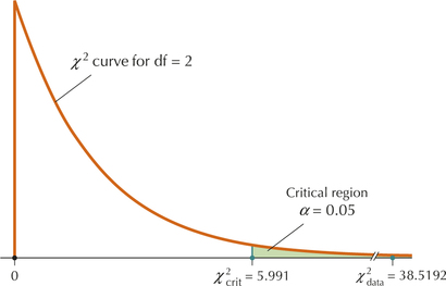
Step 4 State the conclusion and the interpretation. Our $χ_{data}^{2}$ of 38.5192 is greater than our $χ_{crit}^{2}$ of 5.991 (see Figure 16), and so we reject $H_{0}$ . The interpretation is: “There is evidence at level of significance $α = 0.05$ that age group and response are dependent.”
Page 650

FIGURE 16 $χ_{data}^{2} = 38.5192$ lies in the critical region.

NOW YOU CAN DO

Exercises 11–14.

$χ^{2}$ Test for Independence: p-Value Method

Step 1 State the hypotheses and the rejection rule. Check the conditions.
- $H_{0} : Variable A and Variable B are independent$ .
- $H_{a} : Variable A and Variable B are dependent.$ .
Reject $H_{0}$ if the p-value $\leq α$ .

The following conditions must be met:

None of the expected frequencies is less than 1.
At most, 20% of the expected frequencies are less than 5.

The expected frequency for a given cell is

$expected frequency = \frac{(row total) (column total)}{grand total}$

Step 2 Calculate $χ_{data}^{2}$ .

$χ_{data}^{2} = \sum \frac{{(O_{i} - E_{i})}^{2}}{E_{i}}$

where $O_{i} = observed frequency$ and $E_{i} = expected frequency for each cell$ .
Step 3 Find the p-value.

$p -value = P (χ^{2} > χ_{data}^{2})$
Step 4 State the conclusion and the interpretation. Compare the p-value with $α$ .

EXAMPLE 8 $χ^{2}$ test for independence using the p-value method and technology

youngliving

The National Center for Health Statistics publishes information on the living arrangements of America's young people. Table 9 contains a random sample of 200 young people ages 1-24, indicating their gender and living arrangements. Test whether gender and living arrangement are independent, using the TI-83/84, Minitab, JMP, the p-value method, and level of significance $α = 0.10$ .

Table 11.24: Table 9 Contingency table of living arrangements versus gender

	Living arrangements
Gender	Living with parents	Living with partner	All other arrangements	Total
Female	51	22	28	101
Male	58	14	27	99
Total	109	36	55	200

Page 651

Solution

Step 1 State the hypotheses and the rejection rule. Check the conditions.
- $H_{0} : Gender and living arrangements are independent$ .
- $H_{a} : Gender and living arrangements are dependent$ .
Reject $H_{0}$ if the p-value $\leq 0.10$ .

Note that Minitab provides the expected counts (frequencies) below the observed counts. We can then verify that none of the expected frequencies is less than 1, and that none of the expected frequencies has a value less than 5.
Step 2 Calculate $χ_{data}^{2}$ . We use the instructions found in the Step-by-Step Technology Guide at the end of this section. The TI-83/84 results in Figure 17 tell us that $χ_{data}^{2} = 2.225723453$ . The Minitab results in Figure 18 round this to $“Pearson Chi-Square” = χ_{data}^{2} = 2.226$ The JMP results in Figure 19 (“Pearson”) also round this to $“ChiSquare” = χ_{data}^{2} = 2.226$ .

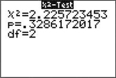FIGURE 17 TI-83/84 $χ^{2}$ results.

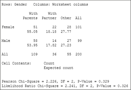FIGURE 18 Minitab $χ^{2}$ results.

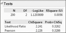FIGURE 19 JMP $χ^{2}$ results.
Step 3 Find the p-value. From the TI-83/84 results in Figure 17, we have

$p -value = P (χ^{2} > χ_{data}^{2}) = 0.3286172017 \approx 0.329.$
Step 4 State the conclusion and the interpretation. Because p-value ≈ 0.329 is not less than level of significance 0.10, we do not reject $H_{0} .$ There is insufficient evidence that gender and living arrangements are dependent.

NOW YOU CAN DO

Exercises 15–18.

3 $χ^{2}$ Test for the Homogeneity of Proportions

Recall the two-sample $Z$ test for $p_{1} - p_{2}$ from Section 10.3, where we compared the proportions of two independent populations. When we extend that hypothesis test to $k$ independent populations, we use a test statistic that follows a $χ^{2}$ distribution. Just as the null hypothesis for the two-sample test assumed no difference between the population proportions

the null hypothesis for the $k$ -sample test also assumes that all $k$ proportions are equal, and
the alternative hypothesis states that not all the population proportions are equal.

When performing the test for the homogeneity of proportions, we use the same steps as for the $χ^{2}$ test for independence.

Page 652

Developing Your Statistical Sense

Difference Between $χ^{2}$ Test for Homogeneity and $χ^{2}$ Test for Independence

The difference between the test for homogeneity of proportions and the test for independence has to do with how the data are collected. If a single sample is taken and two variables are measured, then the test for independence is appropriate.

If several ( $k$ ) samples are taken and the sample proportion is measured for each sample, then the test for homogeneity of proportions is appropriate.

EXAMPLE 9 $χ^{2}$ Test for the homogeneity of proportions

The American Academy of Pediatrics recommends that children's TV-watching time be limited to two hours or less per day. Here, we examine whether a relationship exists between watching TV for more than two hours per day and being overweight. The National Center for Health Statistics conducted a survey of children 12–15 years old. Three random samples were taken, one sample of normal or underweight children, one sample of overweight children, and one sample of obese children. The surveys noted whether the children watched TV more than two hours per day. The results are shown in Table 10.

Test whether the population proportions of children watching more than two hours per day of TV are the same for the three weight statuses, using the p-value method, Minitab, and level of significance $α = 0.05$ .

tvandweight

Table 11.25: Table 10 Numbers watching more than two hours of TV, for three weight statuses

	Normal or underweight	Overweight	Obese	Total
Number watching more than two hours of TV	140	44	82	266
Number watching two hours or less of TV	329	80	91	500
Total	469	124	173	766

Solution

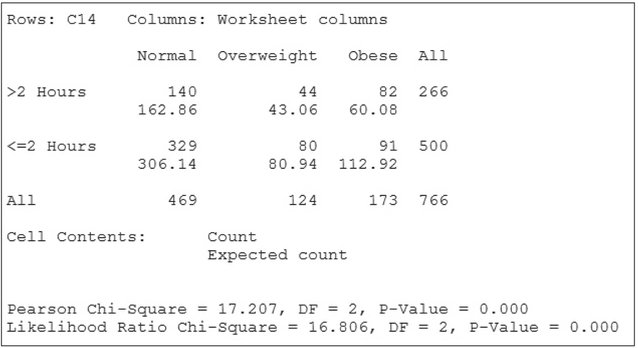
The Minitab results are shown here in Figure 20.

FIGURE 20 Minitab results for the

$χ^{2}$ test for homogeneity.

Page 653

We use the same steps as for the $χ^{2}$ test for independence.

Step 1 State the hypotheses and the rejection rule. Check the conditions.
- $H_{0} : p_{Normal / Under} = p_{Overweight} = p_{Obese}$
- $H_{a} :$ Not all the proportions in $H_{0}$ are equal.
Reject $H_{0}$ if the p-value $\leq 0.05$ .

The expected frequencies are shown in Figure 20. None of them are less than either 1 or 5. Therefore, the conditions are met, and we may proceed with the hypothesis test.

Note: The conditions and the test statistic for the test for the homogeneity of proportions are the same as for the test for independence.
Step 2 Find the test statistic $χ_{data}^{2} • χ_{data}^{2}$ is shown as “Pearson Chi-Square = 17.207.” There are $r = 2$ rows and $c = 3$ columns, so the degrees of freedom are $(r - 1) (c - 1) = (2 - 1) (3 - 1) = 2$ .
Step 3 Find the p-value. Minitab provides the p-value, which is essentially 0.000.
Step 4 State the conclusion and the interpretation. The p-value of 0.000 is less than $α = 0.05$ . We therefore reject $H_{0}$ . Evidence exists, at level of significance $α = 0.05$ , that not all population proportions of watching TV more than two hours per day are equal.

NOW YOU CAN DO

Exercises 19–26.

Online Dating

We look at two tests for independence in this Case Study. The first examines whether the type of relationship reported by respondents depends on the gender of the respondent. The second investigates whether the self-reported physical appearance of online daters depends on the person's gender.

Does the reported Type of relationship Depend on Gender?

The Pew Internet and American Life Project examined whether single men and women differed with respect to their current relationships. The observed frequencies are given in Table 11.

onlinedating

Table 11.26: Table 11 Observed frequencies, online dating study

	Gender
Type of relationship	Single men	Single women
In committed relationship	115	138
Not in committed relationship and not looking for partner	162	391
Not in committed relationship but looking for partner	89	54
Don't know/refused	19	18

We are interested in whether the type of relationship reported depends on the gender of the respondent. In other words, we will test whether the type of relationship is independent of gender. We will use the p-value method, with level of significance $α = 0.05$ , and we will follow the TI-83/84 instructions in the Step-by-Step Technology Guide on page 656 for the calculations.

Page 654

What Results Might We Expect?

Table 11 and Figure 21 indicate that the proportion of men who are “looking” is greater than the proportion of women who are “looking.” Similarly, the proportion of women who are “not looking” is greater than for men. This is evidence that the type of relationship depends on gender and that we might expect to reject the null hypothesis of independence.

FIGURE 21 Graphical evidence indicates type of relationship depends on gender.

Step 1 State the hypotheses and the rejection rule. Check the conditions.
- $H_{0} : Type of relationship and gender are independent$ .
- $H_{a} : Type of relationship and gender are dependent$ .
Reject $H_{0}$ if the p-value $\leq 0.05$ .

Figure 22 shows the expected frequencies, none of which are less than 5. Thus, the conditions are met.

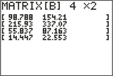FIGURE 22 Expected frequencies.
Step 2 Find $χ_{data}^{2} •$ The TI-83/84 results in Figure 23 tell us

$χ_{data}^{2} = 61.12955651$

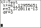FIGURE 23 $χ^{2}$ results on TI-83/84.
Step 3 Find the p-value. Figure 23 also gives us the p-value:

$p -value = 3.372011 E- 13 \approx 0.0000000000003372011$
Step 4 State the conclusion and the interpretation. The p-value $\leq α = 0.05$ , so we reject $H_{0}$ , as we expected. There is evidence that the type of relationship reported in the study depends on the gender of the respondent for level of significance $α = 0.05$ .

Page 655

Does Self-Reported Physical Appearance of Online Daters Depend on Gender?

onlineappear

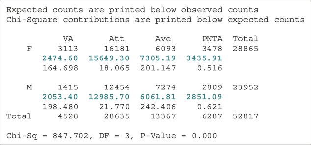
A Master's thesis from the Massachusetts Institute of Technology examined the charonlineappear acteristics and behavior of online daters.⁶ Table 12 contains the self-reported physical appearance and gender of 52,817 users of an online dating service.

Table 11.27: Table 12 Gender and self-reported physical appearance

	Physical appearance
	Very attractive	Attractive	Average	Prefer not to answer	Total
Female	3,113	16,181	6,093	3,478	28,865
Male	1,415	12,454	7,274	2,809	23,952
Total	4,528	28,635	13,367	6,287	52,817

Note from Table 12 that females seem to have higher proportions of those self-reporting as either attractive or very attractive, whereas males seem to have a higher proportion of those self-reporting as average. This is evidence that self-reported physical appearance does depend on gender and that we might expect to reject the null hypothesis of independence. We will test with the p-value method, using level of significance $α = 0.01$ , and Minitab. The hypotheses are

$H_{0} : Self-reported physical appearance and gender are independent$ .
$H_{a} : Self-reported physical appearance and gender are dependent$ .

We reject $H_{0}$ if the p-value ≤ level of significance $α = 0.01$ .

The Minitab results in Figure 24 tell us

$\begin{matrix} χ_{data}^{2} = " Chi - Sq " = 847.702 \\ p -value \approx 0 \end{matrix}$

Figure 24 gives us the expected frequencies (highlighted in color), none of which are less than 5, allowing us to perform the hypothesis test. The p-value $\leq α = 0.01$ , so we reject $H_{0}$ , as we expected. There is evidence at level of significance $α = 0.01$ that the self-reported physical appearance depends on the gender of the online dater.

FIGURE 24 Minitab results showing expected frequencies,

$χ_{data}^{2}$ , and the p-value.

11.2 χ2<math><mrow><msup><mi>χ</mi><mn>2</mn></msup></mrow></math> Tests for Independence and for Homogeneity of Proportions

11.2 $χ^{2}$ Tests for Independence and for Homogeneity of Proportions