12.4 Two-Way ANOVA
OBJECTIVES By the end of this section, I will be able to …
- Construct and interpret an interaction graph.
- Perform a two-way ANOVA.
In Section 12.1, we analyzed the treatment means for a single factor in one-way ANOVA. Then, in Section 12.3, a second factor was introduced, but we were not interested in testing for this blocking factor (or nuisance factor). Finally, here in Section 12.4, we learn about two-way ANOVA, where we are interested in testing for the significance of two factors.
Consumer Reports publishes ratings of many different items, including cell phones and smartphones. Table 9 contains a random sample of the cell phone and smartphone ratings for three leading carriers, AT&T, T-Mobile, and Verizon, published November 15, 2010.
| Phone | Carrier | Type | Rating |
|---|---|---|---|
| Samsung Impression | AT&T | Cell | 68 |
| Pantech Breeze | AT&T | Cell | 62 |
| Samsung Gravity | T-Mobile | Cell | 69 |
| Sony Ericsson | T-Mobile | Cell | 61 |
| Nokia Twist | Verizon | Cell | 66 |
| LG Cosmos | Verizon | Cell | 63 |
| Apple iPhone 4 | AT&T | Smart | 76 |
| Sony Experia | AT&T | Smart | 68 |
| Samsung Vibrant | T-Mobile | Smart | 76 |
| Blackberry Bold | T-Mobile | Smart | 69 |
| Motorola Droid | Verizon | Smart | 75 |
| Blackberry Storm | Verizon | Smart | 70 |
Let us denote carrier as Factor A and type as Factor B, and rating as the response variable. Together, Factor A and Factor B are known as the main effects. We rearrange Table 9 into the 2 × 3 contingency table shown in Table 10. Each cell in the table contains two ratings of carrier/phone type combination as well as the mean of these ratings.
| Factor A: Carrier | ||||
|---|---|---|---|---|
| AT&T | T- Mobile | Verizon | ||
| Factor B: Type | Cell phone | 68 62Mean=65 | 69 61Mean=65 | 66 63Mean=64.5 |
| Smartphone | 76 68Mean=72 | 76 69Mean=72.5 | 75 70Mean=72.5 | |
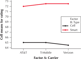
Informally, Table 10 shows that the cell means in a given row do not differ by much. For example, the means in the cell phone row are all roughly 65. In contrast, the cell means in a column do seem to differ somewhat. For example, the column AT&T has means 65 and 72. This hints that “Factor A: Carrier” may not be significant, whereas “Factor B: Type” may have a significant effect on ratings. But we need to perform the actual two-way ANOVA to determine this beyond a reasonable doubt.
1 Constructing and Interpreting an Interaction Graph
Before we perform two-way ANOVA, however, we should ascertain whether factor interaction is present. If the two factors have substantial interaction, then we cannot safely draw conclusions about either factor. So it is important when performing two-way ANOVA to check for the presence of interaction between the factors.
Interaction exists between two factors when the effect of one factor depends on the level of the other factor.
For example, suppose that the mean smartphone ratings for AT&T and T-Mobile were higher than their cell phone ratings, but for Verizon, the cell phone ratings were higher. This would be an example of interaction, because the effect of the type factor (cell phone versus smartphone ratings) depended on the level of the carrier factor.
We investigate the presence of interaction using an interaction plot.
An interaction plot is a graphical representation of the cell means for each cell in the contingency table. To construct an interaction plot:
- Compute the cell means for all cells.
- Construct an x−y plot (Cartesian plane). Label the horizontal axis for each level of Factor A. The vertical axis represents the response variable.
- For the first level of Factor A, insert a point at a height representing the cell means for the response variable, for each level of Factor B. Then do this for the other levels of Factor A.
- Connect points that have a common Factor B level.
EXAMPLE 13 Constructing an interaction plot
mobilephone
Construct the interaction plot for the data in Table 9.
Solution
We have already calculated the cell means in Table 10. We then use the instructions in the Step-by-Step Technology Guide to construct the interaction plot in Minitab, shown here in Figure 37.
NOW YOU CAN DO
Exercises 9–16.
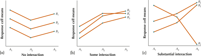
Figure 38 contains some typical interaction plots, showing (a) no interaction, (b) some interaction, and (c) significant interaction, with three levels for each of Factor A and Factor B. In an interaction plot, we are looking to see if the lines are parallel, or nearly parallel, or not at all parallel. Parallel lines indicate no interaction (Figure 38a); nearly parallel lines indicate some interaction (Figure 38b); lines that are not at all parallel indicate substantial interaction (Figure 38c).
2 Performing a Two-Way ANOVA
Next, we turn to performing the two-way ANOVA. The requirements are the same as for one-way ANOVA:
- Random samples are taken from each of k normally distributed populations.
- The variances (σ2) of the populations are all equal.
- The samples are independently drawn.
These requirements may be checked as we did for the one-way ANOVA requirement.
Two-way ANOVA actually involves a series of three hypothesis tests:
- Test for interaction between the factors
- Test for Factor A effect
- Test for Factor B effect
 If interaction between the factors occurs, then we cannot draw conclusions about the main effects. If the test for interaction produces evidence that interaction is present, then do not perform the test for either Factor A or Factor B.
The steps involved in performing a two-way ANOVA are illustrated using the following example.
EXAMPLE 14 Performing a two-way ANOVA
cellsmartphone
Perform a two-way ANOVA for the cell phone and smartphone ratings data in Table 9, using level of significance α=0.05. Assume the requirements are met.
Solution
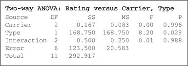
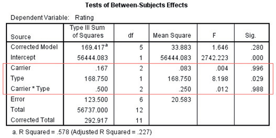
The Minitab results are provided in Figure 39, and the SPSS results are provided in Figure 40.
The null hypothesis H0 in the test for interaction always states that there is no interaction between the factors.
Step 1 Test for interaction. The hypotheses are:
- H0:There is no interaction between carrier (Factor A) and type (Factor B).
- Ha:There is interaction between carrier and type.
Reject H0 if the p-value≤α=0.05. The p-value in the Interaction row in Figure 39 is 0.988, which is not ≤0.05; therefore, do not reject H0. There is insufficient evidence of interaction between carrier and type at level of significance α=0.05. Therefore, we may proceed with the tests for the main effects.
Page 705Step 2 Test for Factor A. The hypotheses are:
- H0:There is no carrier (Factor A) effect. That is, the population mean ratings do not differ by carrier.
- Ha:There is a carrier (Factor A) effect. The population mean ratings do differ by carrier.
Reject H0 if the p-value≤0.05. According to the two-way ANOVA table in Figure 39:
- p-value in the Carrier (Factor A) row = 0.996, which is not ≤0.05
Therefore, we do not reject H0. There is insufficient evidence for a carrier (Factor A) effect. Thus, we do not find a statistically significant difference in Consumer Reports ratings among the three carriers, AT&T, T-Mobile, and Verizon.
Step 3 Test for Factor B. The hypotheses are
- H0:There is no type (Factor B) effect. That is, the population mean ratings do not differ by phone type.
- Ha:There is a type (Factor B) effect. The population mean ratings do differ by phone type.
Reject H0 if the p-value≤0.05. The p-value in the type (Factor B) row in Figure 39 is 0.029, which is ≤0.05; therefore, reject H0. There is evidence for a type (Factor B) effect. Thus, we can conclude that there is significant difference in Consumer Reports ratings between the types: cell phones versus smartphones.
NOW YOU CAN DO
Exercises 17–20.
The next example illustrates what happens when interaction is present.
EXAMPLE 15 Two-way ANOVA when interaction is present
computerrating
Consumer Reports also provides ratings for computers. A random sample of laptop computers and desktop computers from three leading manufacturers, together with the Consumer Reports rating, is shown in Table 11. Table 12 organizes this information into a 2 × 3 contingency table, with three levels of Factor A (company) and two levels of Factor B (type), along with the ratings for each company/type combination, and the cell mean ratings. If appropriate, perform a two-way ANOVA for this data, using level of significance α=0.01. Assume that the requirements are met.
| Computer | Company | Type | Rating |
|---|---|---|---|
| MacBook MC372 | Apple | Laptop | 78 |
| MacBook MC024 | Apple | Laptop | 80 |
| Studio 15 | Dell | Laptop | 72 |
| Inspiron 1545 | Dell | Laptop | 62 |
| Pavilion DV6 | HP | Laptop | 64 |
| G60 | HP | Laptop | 58 |
| iMac MC510 | Apple | Desktop | 73 |
| iMac MC024 | Apple | Desktop | 67 |
| XPS 8100 | Dell | Desktop | 84 |
| XPS 7100 | Dell | Desktop | 80 |
| Pavilion HPE | HP | Desktop | 89 |
| Pavilion Elite | HP | Desktop | 83 |
| Factor A: Company | ||||
|---|---|---|---|---|
| Apple | Dell | HP | ||
| Factor B: Type | Laptop | 78 80Mean=79 | 72 62Mean=67 | 64 58Mean=61 |
| Desktop | 73 67Mean=70 | 84 80Mean=82 | 89 83Mean=86 | |
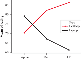
What Result Might We Expect?
The interaction plot in Figure 41 indicates the presence of substantial interaction. We would therefore expect that the test for interaction will find that interaction is present.
Step 1 Test for interaction. The hypotheses are:
- H0:There is no interaction between company (Factor A) and type (Factor B).
- Ha:There is interaction between company and type.
Reject H0 if the p-value≤0.01. The results of the two-way ANOVA are provided in Figure 42.
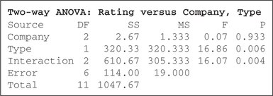
The presence of interaction between the effects makes it problematical to draw conclusions about the factors company and type.
The p-value in the Interaction row in Figure 42 is 0.004, which is ≤0.01; therefore, reject H0. As expected, there is evidence of interaction between company and type at level of significance α=0.01. Therefore, we may not proceed with the tests for the main effects.