12 Analysis of Variance

12.1 One-Way Analysis of Variance (ANOVA)

This page includes Video Technology Manuals

This page includes Statistical Videos

OBJECTIVES By the end of this section, I will be able to …

Explain how analysis of variance works.
Perform one-way analysis of variance.

1 How Analysis of Variance (ANOVA) Works

Analysis of variance (ANOVA) is a hypothesis test for determining whether three or more means of different populations are equal. ANOVA works by comparing the variability between the samples to the variability within the samples.

Suppose we are interested in determining whether significant differences exist in grade point averages (GPAs) among residents of three dormitories, A, B, and C. Table 1 displays three random samples of GPAs of 10 residents from each dormitory.

Table 12.1: Table 1 Sample GPAs from Dorms A, B, and C

A	0.60	3.82	4.00	2.22	1.46	2.91	2.20	1.60	0.89	2.30
B	2.12	2.00	1.03	3.47	3.70	1.72	3.15	3.93	1.26	2.62
C	3.65	1.57	3.36	1.17	2.55	3.12	3.60	4.00	2.85	2.13

The sample mean GPA for Dormitory A is

${\bar{x}}_{A} = \frac{0.60 + 3.82 + 4.00 + 2.22 + 1.46 + 2.91 + 2.20 + 1.60 + 0.89 + 2.30}{10} = 2.2$

Similarly, we can find the sample mean GPAs for the other dormitories: ${\bar{x}}_{B} = 2.5$ and ${\bar{x}}_{C} = 2.8$ . We note that the sample means are not equal. The question is: Are the population means equal? Let $μ_{A}$ , $μ_{B}$ , and $μ_{C}$ represent the population mean GPAs for Dormitories A, B, and C, respectively. We are interested in the following hypotheses, where $μ_{i}$ represents the population mean GPA for dormitory $i$ :

$\begin{array}{l} H_{0} : μ_{A} = μ_{B} = μ_{C} & versus & H_{a} \end{array} : not all the population means are equal$

Sufficient differences in the sample means would represent evidence that the population means were not equal. The question is: What represents “sufficiently” different? We need something to compare against, such as the spread of each sample. One measure of spread or variability is the range:

$range = \max - \min$

We have

$\begin{array}{l} range (Dorm A) = 4.00 - 0.60 = 3.40 \\ range (Dorm B) = 3.93 - 1.03 = 2.90 \\ range (Dorm C) = 4.00 - 1.17 = 2.83 \end{array}$

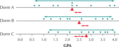
These ranges are rather large spreads, and there is a considerable amount of overlap among the different dormitory GPAs, as shown in Figure 1.

Figure 1 shows the difference among the means for the three dorm GPAs compared with the spread of each dorm's GPAs, as measured by the range. The red triangles represent the sample means, ${\bar{x}}_{A} = 2.2$ , ${\bar{x}}_{B} = 2.5$ , and ${\bar{x}}_{C} = 2.8$ . The spread of the sample means (shown by the red arrows) is much less than the spreads of the individual dorm GPAs (shown by the green arrows). Thus, the sample means ${\bar{x}}_{A} = 2.2$ , ${\bar{x}}_{B} = 2.5$ , and ${\bar{x}}_{C} = 2.8$ are not sufficiently different when compared against the spread of the GPAs. This graph would therefore not provide evidence to reject the null hypothesis that the population mean GPAs are all equal.

Page 667

FIGURE 1 Comparison dotplot of GPAs for Dorms A, B, and C.

Now we make a similar comparison for the GPAs for Dormitories D, E, and F in Table 2.

Table 12.2: Table 2 Sample GPAs from Dorms D, E, and F

D	2.16	2.23	2.09	2.17	2.25	2.19	2.24	2.28	2.25	2.14
E	2.45	2.34	2.58	2.49	2.60	2.42	2.55	2.62	2.45	2.50
F	2.80	2.75	2.93	2.68	2.88	2.75	2.87	2.81	2.73	2.80

The sample mean GPAs for Dormitories D, E, and F are the same as those for Dormitories A, B, and C, respectively: ${\bar{x}}_{D} = 2.2$ , ${\bar{x}}_{E} = 2.5$ , and ${\bar{x}}_{F} = 2.8$ . Again, we are interested in whether the population means are equal.

$\begin{array}{l} H_{0} : μ_{D} = μ_{E} = μ_{F} & versus & H_{a} \end{array} : not all the population means are equal$

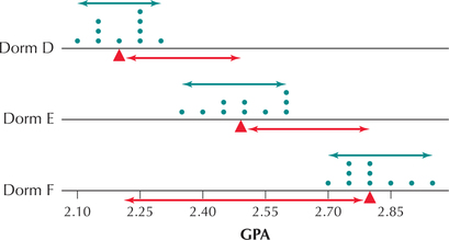
Consider the comparison dotplot in Figure 2. There now seems to be better evidence for concluding that the three population means are not all equal. There is no overlap among the three samples because the spread within each dormitory is much smaller than for Dormitories A, B, and C.

$\begin{array}{l} range (Dorm D) = 2.28 - 2.09 = 0.19 \\ range (Dorm E) = 2.62 - 2.34 = 0.28 \\ range (Dorm F) = 2.93 - 2.68 = 0.25 \end{array}$

Figure 2 shows the difference among the means for the three dorm GPAs compared with the range of each dorm's GPAs. The red triangles represent the sample means, ${\bar{x}}_{D} = 2.2$ , ${\bar{x}}_{E} = 2.5$ , and ${\bar{x}}_{F} = 2.8$ . The spread of the sample means (red arrows) is much greater than the spreads of the individual dorm GPAs (green arrows). Thus, the sample means ${\bar{x}}_{D} = 2.2$ , ${\bar{x}}_{E} = 2.5$ , and ${\bar{x}}_{F} = 2.8$ are sufficiently different when compared against the range of the GPAs. This graph would, therefore, provide some evidence to reject the null hypothesis that the population mean GPAs are all equal.

FIGURE 2 Comparison dotplot of GPAs for Dorms D, E, and F.

Page 668

Note that we arrived at opposite conclusions for the two sets of dormitories, even though the sample means of the first group are identical to the sample means of the second group. Here is the key difference:

The within-sample spreads of Dormitories A, B, and C are large. Compared to these large spreads, the difference in sample means did not seem large.
The within-sample spreads of Dormitories D, E, and F are small. Compared to these small spreads, the difference in sample means did seem large.

These are the types of comparisons that the ANOVA method makes.

Instead of using the range as the measure of spread, analysis of variance uses the standard deviation of the individual samples. Recall that samples with larger spread have larger standard deviations, just as they have larger ranges.

Developing Your Statistical Sense

How Does Analysis of Variance Work?

The key to how analysis of variance works is the following comparison. Compare

the variability in the sample means—that is, how large the differences are between the sample means (indicated by the lengths of the red arrows in Figures 1 and 2)—with
the variability within each sample—that is, the within-sample spreads (indicated by the lengths of the green arrows in Figures 1 and 2).

When (a) is much larger than (b), this is evidence that the population means are not all equal and that we should reject the null hypothesis. Thus, our analysis depends on measuring variability—and hence the term analysis of variance.

Just as for hypothesis-testing procedures from previous chapters, analysis of variance can be performed only if certain requirements are met.

Requirements for Performing Analysis of Variance

Each of the $k$ populations is normally distributed.
The variances $(σ^{2})$ of the populations are all equal.
The samples are independently drawn.

Note: In analysis of variance, the null hypothesis always states that all the population means are equal and the alternative hypothesis always states that not all the population means are equal. Note that $H_{a}$ is not stating that the population means are all different. For $H_{a}$ to be true, it is sufficient for a single population mean to be different, even though all the other population means may be equal.

Our hypotheses for testing for the equality of the population mean GPA for Dormitories A, B, and C are

$\begin{array}{l} H_{0} : μ_{A} = μ_{B} = μ_{C} & versus & H_{a} : not all the population means are equal \end{array}$

Let us stop for a moment to consider what these requirements and the hypotheses mean.

If $H_{0}$ is true, then all three dormitories would have the same population mean GPA: $μ_{A} = μ_{B} = μ_{C} = μ$ , where we denote the hypothesized common mean as $μ$ .
Requirement 1 states that each population is normally distributed.
Requirement 2 states that all the population variances are equal. Let's call this common variance $σ^{2}$ .

Putting all this together, $H_{0}$ assumes that the observations from each population come from the same normal distribution, with mean $μ$ and variance $σ^{2}$ .

Page 669

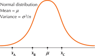
Suppose we then take samples of size $n$ from each group. Fact 3 in Chapter 7 states that the sampling distribution of $\bar{x}$ for a sample of size $n$ taken from a normal population with mean $μ$ and standard deviation $σ$ (that is, variance $σ^{2}$ ) is also normal, with mean $μ$ and standard deviation $σ / \sqrt{n}$ (that is, variance $σ^{2} / \sqrt{n}$ ), as shown in Figure 3. Each dormitory's GPA is assumed (under $H_{0}$ ) to come from the same sampling distribution, so we would expect the sample means to be fairly close together.

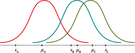
On the other hand, if $H_{0}$ is not true, then not all the population means are equal (Figure 4). In this case, there is no sampling distribution common to all sample means, so we would not expect the sample means to be close together. Note in Figure 4 that each distribution nevertheless has the same shape (normal) and spread (that is, variance) because of the requirements.

FIGURE 3 Common sampling distribution when

$H_{0}$ is true.

FIGURE 4 No common sampling distribution when

$H_{0}$ is not true.

Note: Normal probability plots were introduced in Chapter 7.

Procedure for Verifying the Requirements for Analysis of Variance

Step 1 Normality. Check that the data from each group are normally distributed, using normality probability plots.
Step 2 Equal Variances. Compute the sample standard deviation for each group to verify that the largest standard deviation is not larger than twice the smallest standard deviation.
Step 3 Independence. Verify that the samples drawn from each group are independently drawn.

EXAMPLE 1 Verify the requirements for performing an analysis of variance

dormitory

Verify the requirements for performing an analysis of variance using the hypotheses

$\begin{array}{l} H_{0} : μ_{A} = μ_{B} = μ_{C} & versus & H_{a} : not all the population means are equal \end{array}$

where $μ_{i}$ represents the population mean GPA for Dormitory $i$ , using data from Table 1.

Solution

Step 1 Normality. To verify that each of the $k = 3$ populations is normally distributed, we examine normal probability plots of each sample, shown in Figure 5. Each plot indicates acceptable normality.

FIGURE 5 Normal probability plots verify normality requirement.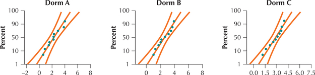

Page 670
Step 2 Equal Variances. To find the standard deviation for Dorm A, we first find

$\begin{array}{l} {\sum {(x - \bar{x})}^{2} = (0.60 - 2.2)}^{2} + (3.82 - 2.2)^{2} + (4.00 - 2.2)^{2} + (2.22 - 2.2)^{2} \\ + (1.46 - 2.2)^{2} + (2.91 - 2.2)^{2} + (2.20 - 2.2)^{2} + (1.60 - 2.2)^{2} \\ + (0.89 - 2.2)^{2} + (2.30 - 2.2)^{2} \\ = 11.5626 \end{array}$

Then

$s_{A} = \sqrt{\frac{\sum {(x - \bar{x})}^{2}}{n - 1}} = \sqrt{\frac{11.5626}{10 - 1}} \approx 1.133460777$

We similarly find $s_{B} \approx 1.030857248$ and $s_{C} \approx 0.9370284$ . The largest, $s_{A} \approx 1.133460777$ , is not larger than twice the smallest, $s_{C} \approx 0.9370284$ . Thus, the equal variance require-ment is satisfied.
Step 3 Independence. Because the students are randomly sampled from each dormitory, with the selection of students in one dormitory not affecting the selection of students sampled from the other dormitories, the independence assumption is also validated.

Note: We retain many decimal places when calculating $s_{A}$ , $s_{B}$ , and $s_{C}$ because these values are used to calculate other quantities later on.

NOW YOU CAN DO

Exercises 7–10.

Note: This form for $\bar{\bar{x}}$ is a weighted mean with the weights being the sample sizes.

Assuming that $H_{0}$ is true, we estimate the common population mean $μ$ using the overall sample mean, $\bar{\bar{x}}$ :

$\bar{\bar{x}} = \frac{(n_{1} {\bar{x}}_{1} + n_{2} {\bar{x}}_{2} + \dots + n_{k} {\bar{x}}_{k})}{n_{t}}$

where there are $k$ samples and $n_{t}$ is the “total sample size” (sum of the $k$ sample sizes). The overall sample mean $\bar{\bar{x}}$ is simply the mean of all the observations from all the samples. For the special case when all the sample sizes are equal, the overall sample mean $\bar{\bar{x}}$ is simply the mean of the $k$ sample means,

$\bar{\bar{x}} = \frac{({\bar{x}}_{1} + {\bar{x}}_{2} + \dots + {\bar{x}}_{k})}{k}$

EXAMPLE 2 Calculating the overall sample mean $\bar{\bar{x}}$

For the sample GPA data given in Table 1 for Dorms A, B, and C, calculate the overall sample mean, $\bar{\bar{x}}$ .

Solution

We have $k = 3$ dormitories, with sample mean GPAs ${\bar{x}}_{A} = 2.2$ , ${\bar{x}}_{B} = 2.5$ , ${\bar{x}}_{C} = 2.8$ . Also, $n_{A} = n_{B} = n_{C} = 10$ , and $n_{t} = 10 + 10 + 10 = 30$ . Thus,

$\bar{\bar{x}} = \frac{10 (2.2) + 10 (2.5) + 10 (2.8)}{30} = 2.5$

All the sample sizes are equal, so we can also calculate $\bar{\bar{x}}$ as follows:

$\bar{x} = \frac{(2.2 + 2.5 + 2.8)}{30} = 2.5$

NOW YOU CAN DO

Exercises 11–14.

Page 671

What Does This Number Mean?

$\bar{\bar{x}} = 2.5$ is the mean GPA for all 30 students from all three samples. We can use $\bar{\bar{x}}$ as our estimate of the common population mean $μ$ assumed in $H_{0}$ .

Recall that analysis of variance works by comparing the variability in the sample means to the variability within each sample. We use the following statistics to measure these variabilities.

The greater the distance between the sample means, the larger the MSTR.

The larger the standard deviation of the $k$ samples, the larger the MSE.

The mean square treatment (MSTR) measures the variability in the sample means. MSTR is the sample variance of the sample means, weighted by sample size.

$MASTR= \frac{\sum n_{i} {({\bar{x}}_{i} - \bar{\bar{x}})}^{2}}{k - 1}$

where $n_{i}$ and ${\bar{x}}_{i}$ are the sample size and mean of the $i$ th sample, $\bar{\bar{x}}$ is the overall sample mean, and there are $k$ populations.

The mean square error (MSE) measures the variability within the samples. MSE is the mean of the sample variances, weighted by sample size.

$MSE= \frac{\sum (n_{i} - 1) s_{i}^{2}}{n_{i} - 1}$

where $n_{i}$ and $s_{i}^{2}$ are the sample size and variance of the $i$ th sample, $n_{t}$ is the total sample size, and there are $k$ populations.

We compare MSTR to MSE by taking the ratio of these two quantities. This ratio MSTR/MSE follows the $F$ distribution that we learned about in Section 10.4.

The student may want to review the characteristics of the $F$ distribution in Section 10.4.

The test statistic for analysis of variance is

$F_{data} = \frac{MSTR}{MSE}$

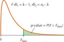
$F_{data}$ measures the variability among the sample means, compared to the variability within the samples. $F_{data}$ follows an $F$ distribution with ${df}_{1} = k - 1$ and ${df}_{2} = n_{t} - k$ , when the following requirements are met: (1) each of the $k$ populations is normally distributed, (2) the variances of the populations are all equal, and (3) the samples are independently drawn.

The term mean square represents a weighted mean of quantities that are squared. Each mean square itself consists of two parts: the sum of squares in the numerator and the degrees of freedom in the denominator. The numerator for MSTR is called the sum of squares treatment (SSTR), and the numerator for MSE is called the sum of squares error (SSE).

$\begin{array}{l} MSTR = \frac{sum of squares treatment}{{df}_{1}} = \frac{SSTR}{{df}_{1}} = \frac{\sum n_{i} {({\bar{x}}_{i} - \bar{\bar{x}})}^{2}}{k - 1} \\ MSE = \frac{sum of squares treatment}{{df}_{2}} = \frac{SSE}{{df}_{2}} = \frac{\sum (n_{i} - 1) s_{i}^{2}}{n_{t} - k} \end{array}$

The total sum of squares (SST) is found by adding SSTR and SSE:

$SST = SSTR + SSE$

The ANOVA table shown in Table 3 is a convenient way to display the various statistics calculated during an analysis of variance. Note that the quantities in the mean square column equal the ratio of the two columns to its left.

Page 672

Table 12.3: Table 3 ANOVA table

Source of variation	Sum of squares	Degrees of freedom	Mean square	$F$ -test statistic
Treatment	SSTR	${df}_{1} = k - 1$	$MSTR = \frac{SSTR}{k - 1}$	$F_{data} = \frac{MSTR}{MSE}$
Error	SSE	${df}_{1} = n_{t} - k$	$MSE = \frac{SSE}{n_{t} - k}$
Total	SST

EXAMPLE 3 Constructing the ANOVA table

Use the summary statistics in Table 4 for the sample GPAs for Dorms A, B, and C to construct the ANOVA table.

Table 12.4: Table 4 Summary statistics for sample GPAs for Dorms A, B, and C

	Dorm A	Dorm B	Dorm C
Mean	${\bar{x}}_{A} = 2.2$	${\bar{x}}_{B} = 2.5$	${\bar{x}}_{C} = 2.8$
Standard deviation	$s_{A} \approx 1.133460777$	$s_{B} \approx 1.030857248$	$s_{C} \approx 09370284$
Sample size	$n_{1} = 10$	$n_{2} = 10$	$n_{3} = 10$

Solution

We have $k = 3$ dormitories, and total sample size $n_{t} = 10 + 10 + 10 = 30$ . Thus,

$\begin{array}{l} SSTR = \sum n_{i} {({\bar{x}}_{i} - \bar{\bar{x}})}^{2} & = 10 {(2.2 - 2.5)}^{2} + 10 {(2.5 - 2.5)}^{2} + 10 {(2.8 - 2.5)}^{2} \\ = 10 [{(- 0.3)}^{2} + {(0)}^{2} + {(0.3)}^{2}] = 1.8 \end{array}$
$\begin{array}{l} SSE & \approx (10 - 1) {(1.33460777)}^{2} + (10 - 1) {(1.030857248)}^{2} + (10 - 1) {(0.9370284)}^{2} \\ \approx 29.0288 \end{array}$
$SST = SSTR + SSE = 1.8 + 29.0288 = 30.8288$
$MSTR = \frac{SSTR}{k - 1} = \frac{1.8}{3 - 1} = 0.9$
$MSE = \frac{SSE}{n_{t} - k} = \frac{29.0288}{30 - 3} = 1.0781407407$
$F_{data} = \frac{MSTR}{MSE} = \frac{0.9}{1.0751407407} = 0.8370997079 \approx 0.84$

We summarize these calculations in the following ANOVA table, with the results rounded for clarity.

Source of variation	Sum of squares	Degrees of freedom	Mean square	$F$ -test statistic
Treatment	SSTR = 1.8	${df}_{1} = 3 - 1 = 2$	$MSTR = \frac{1.8}{2} = 0.9$	$F_{data} = \frac{0.9}{1.075} \approx 0.84$
Error	SSE = 29.0288	${df}_{2} = 30 - 3 = 27$	$MSE = \frac{29.0288}{27} \approx 1.075$
Total	SST = 30.8288

NOW YOU CAN DO

Exercises 15–22.

Page 673

2 Performing One-way ANOVA

Now that we know how it works, we next learn how to perform ANOVA.

Remember: $H_{a}$ is not stating that the population means are all different.

One-way Analysis of Variance

We have taken random samples from each of $k$ populations and want to test whether the population means of the $k$ populations are all equal.

Required conditions:

Each of the $k$ populations is normally distributed.
The variances $(σ^{2})$ of the populations are all equal.
The samples are independently drawn.

Step 1 State the hypotheses, and state the rejection rule.

$\begin{array}{l} H_{0} : μ_{1} = μ_{2} = \dots = μ_{k} & versus & H_{a} \end{array} : not all the population means are equal$

where the $µ's$ represent the population mean from each population. The rejection rule is Reject $H_{0}$ if the $p - v a l u e \leq α$ .
Step 2 Calculate $F_{data}$ .

$F_{data} = \frac{MSTR}{MSE}$

where

$\begin{array}{l} MSTR = \frac{\sum n_{i} {({\bar{x}}_{i} - \bar{\bar{x}})}^{2}}{k - 1} & and & MSE = \frac{\sum (n_{i} - 1) s_{i}^{2}}{n_{t} - k} \end{array}$

$F_{data}$ follows an $F$ distribution with ${df}_{1} = k - 1$ and ${df}_{2} = n_{t} - k$ if the required conditions are satisfied, where $n_{t}$ represents the total sample size.
Step 3 Find the $p$ -value. Use technology to find the $p -value = P (F > F_{data})$ , as shown in Figure 6.
Step 4 State the conclusion and the interpretation. Compare the $p$ -value with $α$ .

FIGURE 6 $p$ -Value for the one-way ANOVA $F$ test.

EXAMPLE 4 Performing one-way ANOVA using the $p$ -value method

Test, using level of significance $α = 0.05$ , whether the population mean GPAs from Example 1 differ among the students in Dormitories A, B, and C.

What Result Might We Expect?

Recall that the comparison dotplot in Figure 1 (page 667) showed a large amount of overlap in the GPAs among dormitories A, B, and C. The large ranges illustrate the large within-dormitory spread of the GPAs for these dorms. When compared against this large within-sample variability, the variability in sample means may not seem large. Therefore, we might expect that the null hypothesis of no difference will not be rejected.

Page 674

Solution

We already verified the requirements for performing the analysis of variance in Example 1.

Step 1 State the hypotheses, and state the rejection rule. Define the $μ_{i}$ .

$\begin{array}{l} H_{0} : μ_{A} = μ_{B} = μ_{C} & versus & H_{a} \end{array} : not all the population means are equal$

where $μ_{i}$ represents the population mean GPA of students from dormitory $i$ . The rejection rule is Reject $H_{0}$ if the $p - v a l u e \leq α = 0.05$ .
Step 2 Calculate $F_{data}$ . From Example 3, we have MSTR = 0.9, MSE = 1.0751407407, and

$F_{data} = \frac{MSTR}{MSE} = \frac{0.9}{1.0751407407} = 0.8370997079$

$F_{data}$ follows an $F$ distribution with ${df}_{1} = k - 1 = 3 - 1 = 2$ and ${df}_{2} = n_{t} - k = 30 - 3 = 27$ .
Step 3 Find the $p$ -value. We use the instructions provided in the Step-by-Step Technology Guide at the end of this section (page 679). From Figures 7 and 8, we have
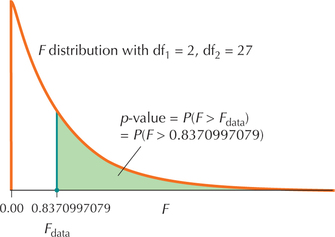$p -value = P (F > F_{data}) = P (F > 0.8370997079) = 0.4438929572 \approx 0.4439$

FIGURE 7 $p -Value = P (F > 0.8370997079)$ .

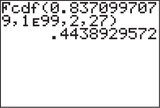FIGURE 8 TI-83/84 $p$ -value.
Step 4 State the conclusion and the interpretation. Compare the $p$ -value with $α$ . The $p$ -value of 0.4439 is not $\leq α = 0.05$ , so we do not reject $H_{0}$ . As expected, there is not enough evidence to conclude at level of significance $α = 0.05$ that not all population mean GPAs are equal.

When calculating the $p$ -value for analysis of variance, always retain as many decimal places in the value of $F_{data}$ as you can. This will make the $p$ -value as accurate as possible. Rounding $F_{data}$ too much will make the $p$ -value less accurate.

NOW YOU CAN DO

Exercises 23–28.

EXAMPLE 5 Performing one-way ANOVA using technology

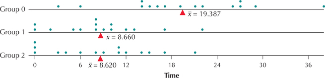
Researchers from the Institute for Behavioral Genetics at the University of Colorado investigated the effect that the enzyme protein kinase C (PKC) has on anxiety in mice. The genotype for a particular gene in a mouse (or a human) consists of two alleles (copies) of each chromosome, one each from the father and mother. The investigators in the study separated the mice into three groups. In Group 0, neither of the mice's alleles for PKC produced the enzyme. In Group 1, one of the two alleles for PKC produced the enzyme and the other did not. In Group 2, both PKC alleles produced the enzyme. To measure the anxiety in the mice, scientists measured the time (in seconds) the mice spent in the “open-ended” sections of an elevated maze. It was surmised that mice spending more time in open-ended sections exhibit decreased anxiety. The data are provided in Table 5. Use technology to test, at $α = 0.01$ , whether the population mean time spent in the open-ended sections of the maze was the same for all three groups.

Page 675

micemaze

Table 12.6: Table 5 Time spent in open-ended section of maze

Group 0		Group 1		Group 2
15.8	14.4	5.2	7.6	10.6	9.2
16.5	25.7	8.7	10.4	6.4	14.5
37.7	26.9	0.0	7.7	2.7	11.1
28.7	21.7	22.2	13.4	11.8	3.5
5.8	15.2	5.5	2.2	0.4	8.0
13.7	26.5	8.4	9.5	13.9	20.7
19.2	20.5	17.2	0.0	0.0	0.0
2.5		11.9		16.5

What Result Might We Expect?

Figure 9 shows a plot of the time in open-ended sections for the mice in the three groups. Note that the Group 1 and Group 2 mice spent on average about the same amount of time in the open-ended sections but that Group 0 spent on average somewhat more time in the open-ended sections. This would tend to suggest that the null hypothesis that all three population means are equal should be rejected. Remember that to reject $H_{0}$ , it is sufficient for just one of the population means to be different.

FIGURE 9 Evidence that the population mean of Group 0 is larger than the others.

Solution

We use the instructions provided in the Step-by-Step Technology Guide at the end of this section (page 679). We frst verify whether the requirements are met.

The normal probability plots in Figure 10 indicate acceptable normality.
The group standard deviations are $s_{0} \approx 9.0$ , $s_{1} \approx 6.0$ , and $s_{2} \approx 6.4$ . Thus, the largest standard deviation is not greater than twice the smaller, which verifies the equal variances requirement.

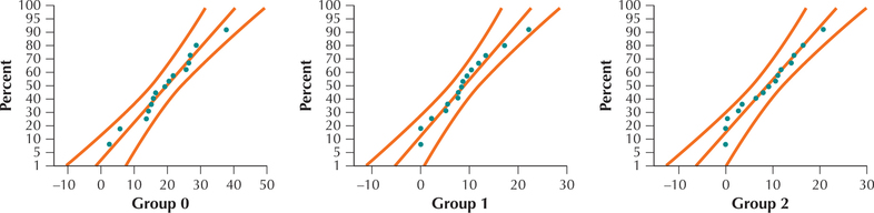FIGURE 10 Normal probability plots.

Page 676
The selection of a mouse to a particular group did not affect the selection of mice to the other groups, so that the samples are independent.

Thus, we proceed with the one-way ANOVA.

$\begin{matrix} H_{0} : μ_{Group 0} = μ_{Group 1} = μ_{Group 2} \\ H_{a} : not all the population means are equal \end{matrix}$

where the $μ's$ represent the population mean time spent in the open-ended sections of the maze for each group.

Figure 11 contains the results from the TI-83/84, showing where each statistic corresponds to the ANOVA table structure in Table 3. We have $F_{data} = 10.906$ , with a $p$ -value of "1.5320224E4" = 0.00015320224. This $p$ -value is less than $α = 0.01$ , so we reject $H_{0}$ . There is evidence at level of significance $α = 0.01$ that the population mean times in the open-ended sections of the maze are not equal for all three groups.

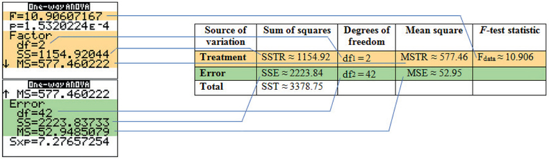
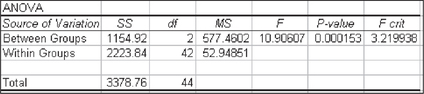
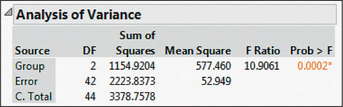
FIGURE 11 Correspondence between TI-83/84 ANOVA output and the ANOVA table.

Figure 12 contains the Excel ANOVA results, Figure 13 contains the Minitab ANOVA results, and Figure 14 contains the JMP ANOVA results. Values differ slightly due to rounding.

FIGURE 12 Excel ANOVA results.

FIGURE 13 Minitab ANOVA results.

FIGURE 14 JMP results.

One-way ANOVA may also be conducted using the critical-value method. The conditions are the same as for the $p$ -value method.

Page 677

EXAMPLE 6 Performing one-way ANOVA using the critical-value method

micemaze

Use the data from Example 5 to test, using the critical-value method and level of significance $α = 0.01$ , whether the population mean time spent in the open-ended sections of the maze was the same for all three groups.

Solution

The conditions for performing ANOVA were verified in Example 5.

Step 1 State the hypotheses.

$\begin{matrix} H_{0} : μ_{Group 0} = μ_{Group 1} = μ_{Group 2} \\ H_{a} : not all the population means are equal \end{matrix}$

where the $μ's$ represent the population mean time spent in the open-ended sections of the maze for each group.
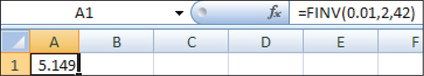
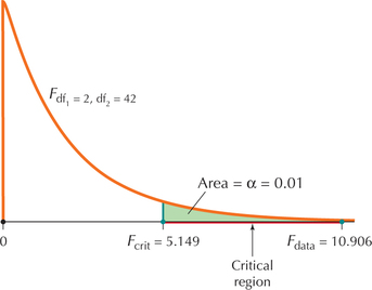
Step 2 Find the critical value $F_{crit}$ and state the rejection rule. The one-way ANOVA test is a right-tailed test, so the $F$ -critical value $F_{crit}$ is the value of the $F$ distribution for ${df}_{1} = k - 1$ and ${df}_{2} = n_{t} - k$ that has area $α$ to the right of it (see Figure 16). Here, ${df}_{1} = 3 - 1 = 2$ and ${df}_{2} = 45 - 3 = 42$ . To find $F_{crit}$ , we may use the F tables or technology. To find our $F_{crit}$ using Excel, enter = FINV(0.01,2,42) in cell A1, as shown in Figure 15. Thus, $F_{crit} = 5.149$ . ANOVA is a right-tailed test, so we will reject $H_{0}$ if $F_{data} ≥ 5.149$ .

FIGURE 15 Using Excel to find the $F$ critical value.
Step 3 Calculate $F_{data}$ . From Example 5, we have $F_{data} = 10.906$ .
Step 4 State the conclusion and interpretation. Because $F_{data} = 10.906 \geq F_{crit} = 5.149$ (Figure 16), we reject $H_{0}$ . There is evidence that not all population mean times spent in the open-ended sections of the maze are equal.

FIGURE 16 $F_{crit} = 5.149$ has area of $α = 0.01$ to the right of it.

NOW YOU CAN DO

Exercises 29–30.

Developing Your Statistical Sense

Do Not Draw the Wrong Conclusion

Note that we did not conclude that all three population means are different. As long as one mean is sufficiently different from the other two, we would reject $H_{0}$ . Our conclusion was simply that the population means were not all equal.

Also, we cannot yet formally conclude that Group 0 has a larger population mean time than the other groups, even though Figure 9 seems to indicate so. All we can formally conclude at this point is that not all the population means are equal. In Section 12.2, we will learn multiple comparisons, which is the type of analysis needed to test whether the mean of Group 0 is larger than the others.

Page 678

Professors on Facebook

A recent study investigated whether the amount of information a professor posts about himself or herself (that is, self-disclosure) on the online social network Facebook is related to student motivation. A professor constructed three different Facebook sites, one offering low self-disclosure, one offering medium self-disclosure, and one offering high self-disclosure. For example, the low-disclosure site offered information only about her position at the university. The medium-disclosure site also showed the professor's favorite movies, books, and quotes. On the high-disclosure site, fictitious comments from “friends” were posted on “the Wall,” highlighting social gatherings.

Study participants (students not enrolled in the professor's courses) were then randomly assigned to access and browse one of the three Facebook sites, develop an impression of the professor, and complete the research questionnaire. Student motivation was measured using a set of 16 items, and the sum of the 16 items was calculated to form the total motivation score. The items measured student interest, involvement, stimulation, level of excitement, and whether the student was inspired or challenged. Use technology to test, at $α = 0.05$ , whether the population mean motivation scores are equal for the three types of Facebook pages: low, medium, and high self-disclosure.

Solution

First, we verify whether the requirements are satisfied.

The normal probability plots in Figure 17 indicate acceptable normality.
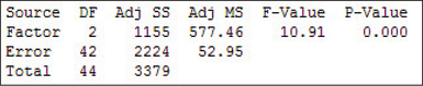
The standard deviations are shown in blue in the Minitab output in Figure 18.
The lamest, $s_{medium} = 14.70$ , is not larger than twice the smallest, $s_{low} = 11.88$ . Thus, the equal-variance requirement is satisfied.
The student participants were randomly selected for each level of self-disclosure, so the independence assumption is also validated.

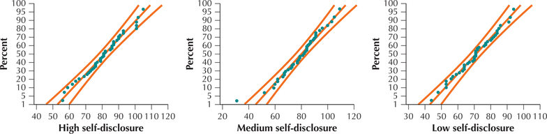FIGURE 17 Normal probability plots.

FIGURE 18 Minitab output for Facebook ANOVA.

Page 679

We therefore proceed with the ANOVA. The hypotheses are

$\begin{array}{l} H_{0} : μ_{high} = μ_{medium} = μ_{low} & versus & H_{a} \end{array} : not all the population means are equal$

where $μ_{i}$ represents a population mean motivation score for each self-disclosure level. Reject $H_{0}$ if the $p$ -value is less than $α = 0.05$ .

From Figure 18, we get $F_{data} = 8.05$ , with an associated $p$ -value of approximately 0.001 (shown in blue). This $p$ -value is less than $α = 0.05$ , so we reject $H_{0}$ . There is evidence that not all population mean motivation scores are equal across all levels of self-disclosure. Informally, we may observe that the mean motivation score for the Facebook Web site with low self-disclosure seems lower than the other groups. We test this formally in Section 2.

The Analysis of Variance applet allows you to experiment with various values for the sample means and the sample variability in order to see how changes in these values affect $F_{data}$ and the $p$ -value.