12.2 Multiple Comparisons
OBJECTIVES By the end of this section, I will be able to …
- Perform multiple comparisons tests using the Bonferroni method.
- Use Tukey's test to perform multiple comparisons.
- Use confidence intervals to perform multiple comparisons for Tukey's test.
Recall Example 5, where we rejected the null hypothesis that the population mean time spent in the open-ended sections of a maze was the same for three groups of genetically altered mice. But so far, we have not tested to find out which pairs of population means are significantly different.
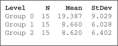
Figure 21 indicates that the sample mean time for Group 0 ˉxGroup 0=19.387 was much larger than the sample means of the other groups ˉxGroup 1=8.660 or ˉxGroup 2=8.620. Because ˉxGroup 0>ˉxGroup 1, and because the ANOVA test produced evidence that the three population means are not equal, we are tempted to conclude that μGroup 0>μGroup 1. However, we cannot formally draw such a conclusion based on the one-way ANOVA results alone. Instead, we need to perform multiple comparisons.
Multiple Comparisons
Once an ANOVA result has been found significant (the null hypothesis is rejected) multiple comparisons procedures seek to determine which pairs of population means are significantly different. Multiple comparisons are not performed if the ANOVA null hypothesis has not been rejected.
We will learn three multiple comparisons procedures: the Bonferroni method, Tukey's test, and Tukey's test using confidence intervals.
1 Performing Multiple Comparisons Tests Using the Bonferroni Method
In Section 10.2, we learned about the independent sample t test for determining whether pairs of population means were significantly different. We will do something similar here, except that (a) the formula for test statistic tdata is different from the one in Section 10.2, and (b) we need to apply the Bonferroni adjustment to the p-value.
Denote the number of population means as k. In general, there are
c=(kC2)=k!2!(k−2)!
possible pairs of means to compare; that is, there are c pairwise comparisons. For k=3, there are c=(3C2)=3!2!(k−2)!=3 comparisons, and for k=4 there are c=(4C2)=4!2!(4−2)!=6 comparisons. We rejected the null hypothesis in Example 5, so we are interested in which pairs of population means are significantly different. There are c=3 hypothesis tests:
- H0:μGroup 0=μGroup 1versusHa:μGroup 0≠μGroup 1
- H0:μGroup 0=μGroup 2versusHa:μGroup 0≠μGroup 2
- H0:μGroup 1=μGroup 2versusHa:μGroup 1≠μGroup 2
Suppose each of these three pairwise hypothesis tests is carried out using a level of significance a=0.05. Then the experimentwise error rate, that is, the probability of making at least one Type I error in these three hypothesis tests is
αEW=1−(1−a)3=0.142625
which is approximately three times larger than α=0.05. The Bonferroni adjustment corrects for this as follows.
Recall that a Type I error is rejecting the null hypothesis when it is true.
The Bonferroni Adjustment
- When performing multiple comparisons, the experimentwise error rate αEW is the probability of making at least one Type I error in the set of hypothesis tests.
- αEW is always greater than the comparison level of significance α by a factor approximately equal to the number of comparisons being made.
- Thus, the Bonferroni adjustment corrects for the experimentwise error rate by multiplying the p-value of each pairwise hypothesis test by the number of comparisons being made. If the Bonferroni-adjusted p-value is greater than 1, then set the adjusted value equal to 1.
For example, when we test H0:μGroup 0=μμGroup 1versusHa:μGroup 0≠μGroup 1, the Bonferroni adjustment says to multiply the resulting p-value by c=3. Example 7 shows how to use the Bonferroni method of multiple comparisons.
EXAMPLE 7 Bonferroni method of multiple comparisons
Use the Bonferroni method of multiple comparisons to determine which pairs of population mean times differ, for the mice in Groups 0, 1, and 2 in Example 5. Use level of significance α=0.01.
Solution
The Bonferroni method requires that
- the requirements for ANOVA have been met, and
- the null hypothesis that the population means are all equal has been rejected.
In Example 5, we verified both requirements.
Step 1 For each of the c hypothesis tests, state the hypotheses and the rejection rule. There are k=3 means, so there will be c=3 hypothesis tests. Our hypotheses are
- Test 1: H0:μGroup 0=μGroup 1versusHa:μGroup 0≠μGroup 1
- Test 2: H0:μGroup 0=μGroup 2versusHa:μGroup 0≠μGroup 2
- Test 3: H0:μGroup 1=μGroup 2versusHa:μGroup 1≠μGroup 2
where μi represents the population mean time spent in the open-ended sections of the maze, for the ith group. For each hypothesis test, reject H0 if the Bonferroni-adjusted p-value≤α=0.01.
Step 2 Calculate tdata for each hypothesis test. From Figure 11 on page 676, we have the mean square error from the original ANOVA as MSE = 52.9485079 and from Figure 21 we get the sample means and the sample sizes. Thus,
- Test 1:
tdata=ˉxGroup 0−ˉxGroup 1√MSE⋅(1nGroup 0+1nGroup 1)=19.387−8.660√(52.9485079)(115+115)≈4.037
- Test 2:
tdata=ˉxGroup 0−ˉxGroup 2√MSE⋅(1nGroup 0+1nGroup 2)=19.387−8.620√(52.9485079)(115+115)≈4.052
- Test 3:
tdata=ˉxGroup 1−ˉxGroup 2√MSE⋅(1nGroup 1+1nGroup 2)=8.660−8.620√(52.9485079)(115+115)≈0.015
When the requirements are met, tdata follows a t distribution with nt−k=45−3=42 degrees of freedom, where nt represents the total sample size.
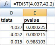 FIGURE 22 Unadjusted p-values from Excel.
- Test 1:
- Step 3 Find the Bonferroni-adjusted p-value for each hypothesis test. Figure 22 shows the unadjusted p-values for the values of tdata from Step 2, using the function tdist (tdata, df,2), where df=42 and the 2 represents a two-tailed test. Then the Bonferroni-adjusted p-value=c⋅(p-value)=3⋅(p-value), for each hypothesis test.Page 688
- Test 1: Bonferroni-adjusted p-value=3⋅0.000225=0.000675.
- Test 2: Bonferroni-adjusted p-value=3⋅0.000215=0.000645.
- Test 3: Bonferroni-adjusted p-value=3⋅0.988103=2.964309, but this value exceeds 1, so we set this p-value equal to 1.
- Step 4 For each hypothesis test, state the conclusion and the interpretation.
- Test 1: The adjusted p-value = , which is ≤0.01; therefore, reject . There is evidence at the 0.01 level of significance that the population mean time spent in the open-ended part of the maze differs between Group 0 and Group 1.
- Test 2: The adjusted , which is ≤0.01; therefore, reject . There is evidence at the 0.01 level of significance that the population mean time differs between Group 0 and Group 2.
- Test 3: The adjusted , which is not ≤0.01; therefore, do not reject . There is insufficient evidence at the 0.01 level of significance that the population mean time differs between Group 1 and Group 2.
NOW YOU CAN DO
Exercises 9–18.
2 Tukey's Test for Multiple Comparisons
We may also use Tukey's test to determine which pairs of population means are significantly different. Tukey's test was developed by John Tukey, whom we met earlier as the developer of the stem-and-leaf display. We illustrate the steps for Tukey's method using an example.
EXAMPLE 8 Tukey's test for multiple comparisons
In the Case Study on page 678, we tested whether the population mean student motivation scores were equal for the three types of professor self-disclosure on Facebook: high, medium, and low. Figure 18 on page 678 contains the ANOVA results, for which we rejected the null hypothesis of equal population mean scores. Use Tukey's method to determine which pairs of population means are significantly different, using level of significance .
Solution
Tukey's method has the same requirements as the Bonferroni method:
- the requirements for ANOVA have been met, and
- the null hypothesis that the population means are all equal has been rejected.
In the Case Study, both requirements were verified.
Step 1 For each of the hypothesis tests, state the hypotheses. There are means, so there will be hypothesis tests. Our hypotheses are:
- Test 1:
- Test 2:
- Test 3:
where represents the population mean score, for the th category.
Step 2 Find the Tukey critical value and state the rejection rule. The total sample size is . Use experimentwise error rate , degrees of freedom , and . Using the table of Tukey critical values (Table G in the Appendix), we seek on the left, but, when we don't find it, we conservatively choose df = 120. Then, in the column for , we find the Tukey critical value (Figure 23). The rejection rule for the Tukey method is “Reject ,” that is, Reject if .
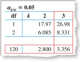 FIGURE 23 Finding the Tukey critical value .Page 689
- Step 3 Calculate the Tukey test statistic for each hypothesis test. From Figure 18 on page 678, we get the sample means, the sample sizes, and the mean square error MSE = 168. Thus,
- Test 1:
- Test 2:
- Test 3:
- Test 1:
- Step 4 For each hypothesis test, state the conclusion and the interpretation.
- Test 1: , which is not ; therefore, do not reject . There is insufficient evidence at the 0.05 level of significance that the population mean student motivation scores differ between professors having high and medium self-disclosure on Facebook.
- Test 2: , which is ; therefore, reject . There is evidence at the 0.05 level of significance that the population mean scores differ between high and low professor self-disclosure on Facebook.
- Test 3: , which is ; therefore, reject . There is evidence at the 0.05 level of significance that the population mean scores differ between medium and low professor self-disclosure on Facebook.
This set of three hypothesis tests has an experimentwise error rate .
When calculating the numerator of for each pairwise comparison, be sure to subtract the smaller value of from the larger value of , so that the value of is positive.
NOW YOU CAN DO
Exercises 19–30.
3 Using Confidence Intervals to Perform Tukey's Test
Tukey's test for multiple comparisons may also be performed using confidence intervals and technology. Recall that when using confidence intervals for hypothesis tests, is rejected if the hypothesized value of the population mean does not fall inside the confidence interval.
Rejection Rule for Using Confidence Intervals to Perform Tukey's test
If a confidence interval for contains zero, then at level of significance , we do not reject the null hypothesis . If the interval does not contain zero, then we do reject .
We illustrate the concept of using confidence intervals to perform Tukey's test with an example using the Facebook data.
EXAMPLE 9 Using confidence intervals to perform Tukey's test
Use the 95% confidence intervals for the differences in population means provided by Minitab to perform Tukey's test for multiple comparisons on the Facebook data.
Solution
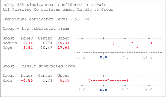
We use the steps in the Step-by-Step Technology Guide provided at the end of this section. Figure 24 contains the output from Minitab showing 95% confidence intervals for the differences in population means for the high, medium, and low professor disclosure levels. The output states that “Group = Low” is being subtracted from the other two groups, meaning that the first two confidence intervals are for and . Later, “Group = Medium” is subtracted from the high group, indicating a confidence interval for . The column headings “Lower” and “Upper” represent the lower and upper bounds of the confidence interval. Figure 25 shows the output from JMP, including 95% confidence intervals for the differences in population means. The output states that the second level listed is subtracted from the first, meaning that the first two confidence intervals are for and . The columns “Lower CL” and “Upper CL” represent the lower and upper bounds of each confidence interval.
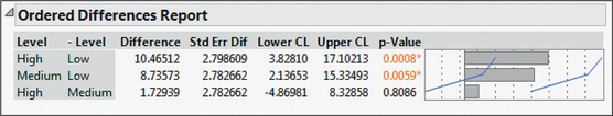
Thus, for our hypothesis tests, we have
Test 1:
95% confidence interval for is (2.14, 15.33), which does not contain zero, so we reject for level of significance .
Test 2:
95% confidence interval for is (3.84, 17.09), which does not contain zero, so we reject for level of significance .
Page 691Test 3:
95% confidence interval for is (–4.86, 8.32), which does contain zero, so we do not reject for level of significance .
Note that these conclusions are exactly the same as the conclusions from Example 8.
NOW YOU CAN DO
Exercises 31 and 32.