10 Two-Sample Inference

10.2 Inference for Two Independent Means

This page includes Statistical Videos

OBJECTIVES By the end of this section, I will be able to …

Perform and interpret $t$ tests about $μ_{1} - μ_{2}$ using Welch's method.⁵
Compute and interpret $t$ intervals for $μ_{1} - μ_{2}$ using Welch's method.
Use confidence intervals for $μ_{1} - μ_{2}$ to perform two-tailed $t$ tests about $μ_{1} - μ_{2}$ .
Perform and interpret $t$ tests and $t$ intervals about $μ_{1} - μ_{2}$ using the pooled variance method.
Apply $Z$ tests and $Z$ intervals for $μ_{1} - μ_{2}$ when $σ_{1}$ and $σ_{2}$ are known.

1 Independent Sample $t$ test for $μ_{1} - μ_{2}$

On page 178 in Chapter 3, we used boxplots to find evidence of a difference between male and female body temperature for a sample of 65 women and a sample of 65 men.⁶ The summary statistics are shown in Table 7.

Table 10.19: Table 7 Summary statistics for female versus male body temperatures in °F

Gender	Sample size	Sample mean body temperature	Sample standard deviation	Population mean body temperature
Females (sample 1)	$n_{1} = 65$	${\bar{x}}_{1} = 98.394$	$s_{1} = 0.743$	$μ_{1} = ?$
Males (sample 2)	$n_{2} = 65$	${\bar{x}}_{2} = 98.105$	$s_{2} = 0.699$	$μ_{2} = ?$

However, because the female subjects did not determine the male subjects, and vice versa, the 65 women and 65 men represent independent samples, so we cannot use the dependent sampling methods we learned in Section 10.1.

Note that for independent samples, we have two sample sizes, $n_{1}$ and $n_{2}$ ; two sample means, ${\bar{x}}_{1}$ and ${\bar{x}}_{2}$ ; two sample standard deviations, $s_{1}$ and $s_{2}$ ; and two unknown population means, $μ_{1}$ and $μ_{2}$ . We are interested in the difference in the population means, so we consider the quantity

$μ_{1} - μ_{2}$

Page 590

Developing Your Statistical Sense

The Difference Difference

A difference in interpretation exists between the quantity $μ_{1} - μ_{2}$ and the quantity $μ_{d}$ from Section 10.1. Here, $μ_{1} - μ_{2}$ refers to the difference in population means, whereas $μ_{d}$ represents the population mean of the paired differences.

In previous chapters, we used the statistic $\bar{x}$ to learn about the parameter $μ$ . Here, we will use the statistic ${\bar{x}}_{1} - {\bar{x}}_{2}$ to perform inference about the parameter $μ_{1} - μ_{2}$ , whose value is unknown. Note from Table 7 that the value of ${\bar{x}}_{1} - {\bar{x}}_{2}$ for these samples is

${\bar{x}}_{1} - {\bar{x}}_{2} = 98.394 - 98.105 = 0.289$

We use ${\bar{x}}_{1} - {\bar{x}}_{2} = 0.289$ as a point estimate of $μ_{1} - μ_{2}$ . If we repeat the experiment an infinite number of times, then the values of ${\bar{x}}_{1} - {\bar{x}}_{2}$ will form a distribution called the sampling distribution of ${\bar{x}}_{1} - {\bar{x}}_{2}$ .

It is unlikely that the experimenter will have knowledge of both population standard deviations $σ_{1}$ and $σ_{2}$ . Therefore, we use the estimates of $σ_{1}$ and $σ_{2}$ provided by the sample standard deviations $s_{1}$ and $s_{2}$ . Recall from Section 8.2 that, when the population standard deviation σ is unknown, and if either the population is normally distributed or the sample size is large, the quantity

$t = \frac{\bar{x} - μ}{s / \sqrt{n}}$

has a $t$ distribution with $n - 1$ degrees of freedom. By analogy, we have the following sampling distribution.

Sampling Distribution of ${\bar{x}}_{1} - {\bar{x}}_{2}$

When random samples are drawn independently from two populations with population means $μ_{1}$ and $μ_{2}$ , and either (a) the two populations are normally distributed, or (b) the two sample sizes are large (at least 30), then the quantity

$t = \frac{({\bar{x}}_{1} - {\bar{x}}_{2}) (μ_{1} - μ_{2})}{\sqrt{\frac{s_{1}^{2}}{n_{1}} + \frac{s_{2}^{2}}{n_{2}}}}$

approximately follows a $t$ distribution with degrees of freedom equal to the smaller of $n_{1} - 1$ and $n_{2} - 1$ , where ${\bar{x}}_{1}$ and $s_{1}$ represent the mean and standard deviation of the sample taken from population 1, and ${\bar{x}}_{2}$ and $s_{2}$ represent the mean and standard deviation of the sample taken from population 2.

This $t$ statistic is called Welch's approximate t, after the twentieth-century English statistician Bernard Lewis Welch. Although there are other distributions that statisticians use to estimate the difference between two population means, we use this approximation because it is conservative and easy to calculate.

Researchers are often interested in testing whether the mean of one population is greater than, less than, or different from the mean of another population. Thus, we next learn how to perform hypothesis tests for the difference in population means $μ_{1} - μ_{2}$ . Usually, the most important hypothesized value for $μ_{1} - μ_{2}$ is 0. Consider the two-tailed hypothesis test

$\begin{matrix} H_{0} : μ_{1} - μ_{2} = 0 & versus & H_{a} : μ_{1} - μ_{2} \neq 0 \end{matrix}$

which is equivalent to

$\begin{matrix} H_{0} : μ_{1} = μ_{2} & versus & H_{a} : μ_{1} \neq μ_{2} \end{matrix}$

In practice, the hypothesized difference between the two population means is nearly always ${(μ_{1} - μ_{2})}_{0} = 0$ . Thus, the test statistic takes the following form:

Page 591

$t_{data} = \frac{({\bar{x}}_{1} - {\bar{x}}_{2}) - 0}{\sqrt{\frac{s_{1}^{2}}{n_{1}} + \frac{s_{2}^{2}}{n_{2}}}} = \frac{({\bar{x}}_{1} - {\bar{x}}_{2})}{\sqrt{\frac{s_{1}^{2}}{n_{1}} + \frac{s_{2}^{2}}{n_{2}}}}$

Just as in Section 9.4, if $t_{data}$ is extreme, then it represents evidence against the null hypothesis. The hypothesis test may be performed using either the critical-value method or the $p$ -value method.

Welch's Hypothesis Test for the Difference in Two Population Means: Critical-Value Method

The hypothesis test applies whenever either

Both populations are normally distributed, or
Both samples are large, that is, $n_{1} \geq 30$ and $n_{2} \geq 30$ .

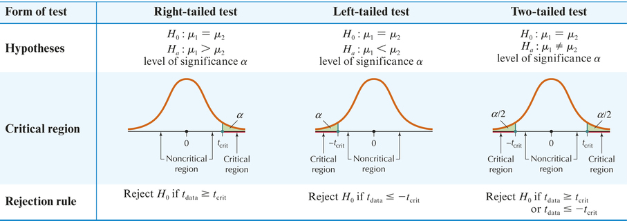
Step 1 State the hypotheses.

Use one of the forms from Table 8. State the meaning of $μ_{1}$ and $μ_{2}$ .
Step 2 Find $t_{crit}$ and state the rejection rule.

To find $t_{crit}$ , use the $t$ table and degrees of freedom the smaller of $n_{1} - 1$ and $n_{2} - 1$ . To find the rejection rule, use Table 8.
Step 3 calculate $t_{data}$ .

$t_{data} = \frac{({\bar{x}}_{1} - {\bar{x}}_{2})}{\sqrt{\frac{s_{1}^{2}}{n_{1}} + \frac{s_{2}^{2}}{n_{2}}}}$

which follows an approximate $t$ distribution with degrees of freedom the smaller of $n_{1} - 1$ and $n_{2} - 1$ .
Step 4 State the conclusion and the interpretation.

Compare $t_{data}$ with $t_{crit}$ .

Table 10.20: Table 8 Critical regions and rejection rules for

$t$ test for

$μ_{1} - μ_{2}$

EXAMPLE 7 $t$ Test for $μ_{1} - μ_{2}$ : Critical-value method

Using Table 7, test whether women's population mean body temperature differs from that of men, using the critical-value method and $α = 0.05$ .

Solution

Both sample sizes are large ( $n_{1} = n_{2} = 65 \geq 30$ ), so we can perform the hypothesis test.

Page 592

Step 1 State the hypotheses.

The key words “differs from” indicate a two-tail test:

$\begin{matrix} H_{0} : μ_{1} = μ_{2} & versus & H_{a} : μ_{1} \neq μ_{2} \end{matrix}$

where $μ_{1}$ and $μ_{2}$ represent the population mean body temperature for women and men, respectively.
Step 2 Find $t_{crit}$ and state the rejection rule.

The required degrees of freedom is the smaller of $n_{1} - 1$ and $n_{2} - 1$ , which is $65 - 1 = 64$ . Unfortunately, $df = 64$ is not in the $t$ table in Appendix Table D, so we use the conservative $df = 60$ . For $α = 0.05$ , this gives $t_{crit} = 2.000$ . We have a two-tailed test, so Table 8 gives us the following rejection rule:

$Reject H_{0} if t_{data} \geq 2.000 or t_{data} \leq - 2.000$
Step 3 Find $t_{data}$ .
$t_{data} = \frac{({\bar{x}}_{1} - {\bar{x}}_{2})}{\sqrt{\frac{s_{1}^{2}}{n_{1}} + \frac{s_{2}^{2}}{n_{2}}}} = \frac{(98.394 - 98.105)}{\sqrt{\frac{{(0.743)}^{2}}{65} + \frac{{(0.699)}^{2}}{65}}} \approx 2.28$
Step 4 State the conclusion and the interpretation.

The test statistic $t_{data} = 2.28$ is greater than $t_{crit} = 2.000$ (see Figure 11). We therefore reject $H_{0}$ . There is evidence, at level of significance $α = 0.05$ , that the population mean body temperatures are not the same for women and men.

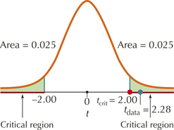FIGURE 11 $t_{data} = 2.28$ falls within the critical region.

NOW YOU CAN DO

Exercises 3–6.

We may also use the $p$ -value method to perform the independent sample $t$ test for $μ_{1} - μ_{2}$ .

Welch's Hypothesis Test for the Difference in Two Population Means: $p$ -value Method

The hypothesis test applies whenever either

Both populations are normally distributed, or
Both samples are large, that is, $n_{1} \geq 30$ and $n_{2} \geq 30$ .

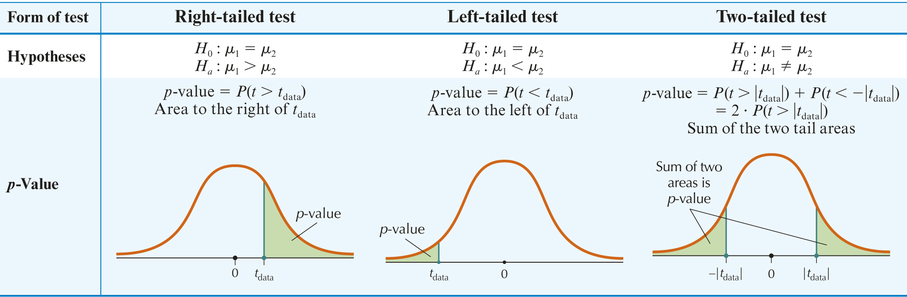
Step 1 State the hypotheses and the rejection rule.

Use one of the forms from Table 9. State the meaning of $μ_{1}$ and $μ_{2}$ . The rejection rule is: Reject $H_{0}$ if the $p$ -value is $\leq α$ .
Step 2 Calculate $t_{data}$ .

$t_{data} = \frac{({\bar{x}}_{1} - {\bar{x}}_{2})}{\sqrt{\frac{s_{1}^{2}}{n_{1}} + \frac{s_{2}^{2}}{n_{2}}}}$

which follows an approximate $t$ distribution with degrees of freedom the smaller of $n_{1} - 1$ and $n_{2} - 1$ .
Step 3 Find the $p$ -value.

Use technology or estimate using the $t$ table.
Step 4 State the conclusion and the interpretation.

Compare the $p$ -value with $α$ .

Page 593

Table 10.21: Table 9

$p$ -Values for t test for

$μ_{1} - μ_{2}$

EXAMPLE 8 $t$ Test for $μ_{1} - μ_{2}$ using the $p$ -value method

bankloan_approved

bankloan_denied

Note: Our degrees of freedom, the smaller of $n_{1} - 1$ and $n_{2} - 1$ , is $100 - 1 = 99$ . However, the TI-83/84 output on the next page shows $df = 143.2490465$ . Why does the technology use different degrees of freedom than we do? Recall that we are using Welch's approximation to the $t$ distribution. The TI-83/84, Excel, Minitab, and other technology calculate the degrees of freedom as follows:⁷

$d f = \frac{{(\frac{s_{1}^{2}}{n_{1}} + \frac{s_{2}^{2}}{n_{2}})}^{2}}{\frac{{(\frac{s_{1}^{2}}{n_{1}})}^{2}}{n_{1} - 1} + \frac{{(\frac{s_{2}^{2}}{n_{2}})}^{2}}{n_{2} - 1}}$

This provides a more accurate determination of the degrees of freedom than our method. However, our method is a conservative estimate that is easier to calculate, and it is recommended for hand calculations.

Bank Loans

Here, we do some analysis on our Chapter 10 Case Study data set: Bank loans. When evaluating loan applicants for approval of a loan, banks examine several aspects of an applicant's financial history. Of particular importance is the applicant's credit score. Here, we will look for differences in the mean credit score between applicants who were approved and those who were denied. Independent samples of size 100 were taken from the Bank loans data set, from among those approved and those denied the loan. The descriptive statistics for each group are shown in Table 10. Use the TI-83/84 or Excel, the $p$ -value method, and level of significance $α = 0.01$ to test whether the population mean credit score for successful loan applicants is greater than that for those who were denied the loan.

Table 10.22: Table 10 Summary statistics for credit scores of loan applicants who were approved and those who were denied the loan

Loan Status	Sample size	Sample mean credit score	Sample standard deviation	Population mean credit score
Approved (sample 1)	$n_{1} = 100$	${\bar{x}}_{1} = 708$	$s_{1} = 34$	$μ_{1} = ?$
Denied (sample 2)	$n_{2} = 100$	${\bar{x}}_{2} = 635$	$s_{2} = 70$	$μ_{2} = ?$

Table 10.22: Source: Data Mining and Predictive Analytics, by Daniel Larose and Chantal Larose, Wiley, 2015.

Solution

Because both samples are large ( $n_{1} = n_{2} = 100 \geq 30$ ), we may proceed with the $t$ test for $μ_{1} - μ_{2}$ .

Page 594

Step 1 State the hypotheses and the rejection rule.

The approved applicants represent sample 1, and we are interested in whether the mean credit score for the approved applicants is greater than that of the denied applicants. Thus, we have the following hypotheses:

$\begin{matrix} H_{0} : μ_{1} = μ_{2} & versus & H_{a} : μ_{1} > μ_{2} \end{matrix}$

where $μ_{1}$ and $μ_{2}$ represent the population mean credit score for the approved and denied loan applicants, respectively. The rejection rule is to reject $H_{0}$ if $p$ -value ≤ 0.01.
Step 2 Find $t_{data}$ .

We use the instructions provided in the Step-by-Step Technology Guide at the end of this section. From Figure 12,

$t_{data} = \frac{({\bar{x}}_{1} - {\bar{x}}_{2})}{\sqrt{\frac{s_{1}^{2}}{n_{1}} + \frac{s_{2}^{2}}{n_{2}}}} \approx \frac{(708 - 635)}{\sqrt{\frac{34^{2}}{100} + \frac{70^{2}}{100}}} \approx 9.38$

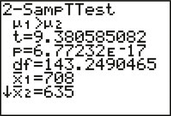FIGURE 12 TI-83/84 output.
Step 3 Find the $p$ -value.

From Figure 12,

$p - value = P (t > t_{data}) = P (t > 9.38) \approx 0.0000000000000000677 \approx 0$
Step 4 State the conclusion and the interpretation.

Our $p$ -value of essentially zero is smaller than the level of significance 0.01. Therefore, we reject $H_{0}$ . There is evidence that the population mean credit score for approved applicants is greater than that of the denied loan applicants. In fact, with a $p$ -value so close to zero, the evidence is very strong indeed.

Remember that when the TI calculator gives you output such as “E-17,” it is indicating that the decimal point needs to be moved 17 places to the left.

NOW YOU CAN DO

Exercises 7–10.

2 $t$ Confidence Intervals for $μ_{1} - μ_{2}$

Recall from Section 8.2 that to estimate the unknown population mean $μ$ , we can use a $t$ confidence interval:

$\bar{x} \pm E = \bar{x} \pm t_{α / 2} (s / \sqrt{n})$

where $E$ is the margin of error. By analogy, here the $t$ interval for $μ_{1} - μ_{2}$ takes the following form.

Welch's Confidence Interval for $μ_{1} - μ_{2}$

For two independent random samples taken from two populations with population means $μ_{1}$ and $μ_{2}$ , a $100 (1 - α) %$ confidence interval for $μ_{1} - μ_{2}$ is given by

$({\bar{x}}_{1} - {\bar{x}}_{2}) \pm t_{α / 2} \sqrt{\frac{s_{1}^{2}}{n_{1}} + \frac{s_{2}^{2}}{n_{2}}}$

where ${\bar{x}}_{1}$ , $s_{1}$ , and $n_{1}$ represent the mean, standard deviation, and sample size of the sample taken from population 1, ${\bar{x}}_{2}$ , $s_{2}$ , and $n_{2}$ represent the mean, standard deviation, and sample size of the sample taken from population 2, and $t_{α / 2}$ is associated with the confidence level and degrees of freedom of the smaller of $n_{1} - 1$ and $n_{2} - 1$ .

The $t$ interval applies whenever either of the following conditions is met:

Both populations are normally distributed, or
Both sample sizes are large.

Margin of Error $E$

The margin of error for a $100 (1 - α) %$ confidence interval for $μ_{1} - μ_{2}$ is given by

$E = t_{α / 2} \cdot \sqrt{\frac{s_{1}^{2}}{n_{1}} + \frac{s_{2}^{2}}{n_{2}}}$

Page 595

Thus, the confidence interval for $μ_{1} - μ_{2}$ takes the form $({\bar{x}}_{1} - {\bar{x}}_{2}) \pm E$ .

This is a confidence interval for the difference in two population means, which is not the same as in Section 10.1, which was for the population mean of the differences of matched pairs. Here, we calculate the means of the samples and then compute the difference. In Section 10.1, we calculated the differences of sample values first and then computed the mean of these differences.

EXAMPLE 9 Confidence interval for $μ_{1} - μ_{2}$

Bank Loans

Find a 90% confidence interval for the difference in population mean credit scores for those approved and those denied bank loans, using the data in Table 10.

Solution

Both sample sizes are large ( $(n_{1} = n_{2} = 100 \geq 30)$ ), so we may construct the interval. For $t_{α / 2}$ , the required degrees of freedom is the smaller of $n_{1} - 1$ and $n_{2} - 1$ , which is $100 - 1 = 99$ . Because $df = 99$ is not listed in the $t$ table, we use the next lower value listed as a conservative alternative: $df = 90$ . For 90% confidence, then $t_{α / 2} = 1.662$ .

The margin of error is

$E = t_{α / 2} \cdot \sqrt{\frac{s_{1}^{2}}{n_{1}} + \frac{s_{2}^{2}}{n_{2}}} \approx (1.662) \cdot \sqrt{\frac{{(34)}^{2}}{100} + \frac{{(70)}^{2}}{100}} \approx 12.934$

The 90% confidence interval is then

$({\bar{x}}_{1} - {\bar{x}}_{2}) \pm E = (708 - 635) \pm 12.934 = (60.066, 85.934)$

We are 90% confident that the difference in population mean credit scores $μ_{1} - μ_{2}$ lies between 60.066 and 85.934. Because 0 is not contained in this interval, we may conclude that $μ_{1} \neq μ_{2}$ , just as we did in Example 8.

NOW YOU CAN DO

Exercises 11–16.

3 Using Confidence Intervals to Perform Hypothesis Tests

As in earlier sections, we may use a $100 (1 - α) %$ $t$ confidence interval for $μ_{1} - μ_{2}$ to perform two-tailed $t$ tests about $μ_{1} - μ_{2}$ .

Equivalence of a Two-Tailed $t$ Test About $μ_{1} - μ_{2}$ and a $t$ Confidence Interval for $μ_{1} - μ_{2}$

If a certain value for $μ_{1} - μ_{2}$ lies outside the corresponding $100 (1 - α) %$ $t$ confidence interval for $μ_{1} - μ_{2}$ , then the null hypothesis specifying this value would be rejected for level of significance $α$ .
Alternatively, if a certain value for $μ_{1} - μ_{2}$ lies inside the $100 (1 - α) %$ $t$ confidence interval for $μ_{1} - μ_{2}$ , then the null hypothesis specifying this value would not be rejected for level of significance $α$ .

EXAMPLE 10 Using a $t$ confidence interval to perform a two-tailed $t$ test about $μ_{1} - μ_{2}$

Bank Loans

Use the 90% confidence interval for the difference in population mean credit scores $μ_{1} - μ_{2}$ from Example 9 to test, using level of significance $α = 0.10$ , whether $μ_{1} - μ_{2}$ differs from the following values:

Page 596

Solution

The hypotheses for our two-sample $t$ test look like this:

$\begin{matrix} H_{0} : μ_{1} = μ_{2} & versus & H_{a} : μ_{1} \neq μ_{2} \end{matrix}$

which is equivalent to the following, if we subtract $μ_{2}$ from each side of the equations:

$\begin{matrix} H_{0} : μ_{1} - μ_{2} = 0 & versus & H_{a} : μ_{1} - μ_{2} \neq 0 \end{matrix}$

Here, we replace zero with the value of 60 hypothesized for the difference in population means, obtaining

$\begin{matrix} H_{0} : μ_{1} - μ_{2} = 60 & versus & H_{a} : μ_{1} - μ_{2} \neq 60 \end{matrix}$

The value of 60 lies outside the confidence interval (60.066, 85.934) from Example 9; therefore, we reject $H_{0}$ .
Our hypotheses are

$\begin{matrix} H_{0} : μ_{1} - μ_{2} = 70 & versus & H_{a} : μ_{1} - μ_{2} \neq 70 \end{matrix}$

The value of 70 lies inside the confidence interval (60.066, 85.934); therefore, we do not reject $H_{0}$ .

NOW YOU CAN DO

Exercises 17–20.

4 $t$ Inference for $μ_{1} - μ_{2}$ Using Pooled Variance

Recall that the variance equals the square of the standard deviation.

An alternative method for $t$ inference may be applied when the data analyst has reason to believe that $σ_{1}^{2} = σ_{2}^{2}$ , that is, the variances of the two populations are equal. A pooled estimate $s_{pooled}^{2}$ of the common variance $σ_{1}^{2} = σ_{2}^{2} = σ^{2}$ is used.

Pooled estimate of the Common Variance $σ^{2}$

$s_{pooled}^{2} = \frac{(n_{1} - 1) s_{1}^{2} + (n_{2} - 1) s_{2}^{2}}{n_{1} + n_{2} - 2}$

Some statisticians think that the pooled variance method should be used sparingly.⁸

The conditions for performing $t$ inference using pooled variance are the same as for Welch's method (page 591), with the additional condition that $σ_{1}^{2} = σ_{2}^{2}$ . The test statistic $t_{data}$ for the pooled variance $t$ test is then given by

$t_{data} = \frac{({\bar{x}}_{1} - {\bar{x}}_{2})}{\sqrt{s_{pooled}^{2} (\frac{1}{n_{1}} + \frac{1}{n_{2}})}}$

We illustrate the pooled variance $t$ test and the pooled variance $t$ confidence interval using the following two examples.

EXAMPLE 11 Pooled variance $t$ test

Bank Loans

Another indicator of financial health that banks look at when evaluating loan applicants is the debt-to-income ratio, which is defined as follows.

$Debt-to-income ratio = \frac{Applicant's total debt}{Applicant's annual income}$

For example, if you owed $5000 on your credit card and $10,000 on your car, and your annual income was $50,000, then your debt-to-income ratio would be $($ 5000 + $ 10, 000) / $ 50, 000 = 0.3$ .

Page 597

Here, we examine whether the mean debt-to-income ratio differed between those approved and those denied the bank loans. Samples of size 100 were obtained from each group, with the summary statistics shown in Table 11.

Table 10.23: Table 11 Summary statistics for debt-to-income ratios of loan applicants who were approved and those who were denied the loan

Loan status	Sample size	Sample mean debt-to-income ratio	Sample standard deviation	Population mean debt-to-income ratio
Approved (sample 1)	$n_{1} = 100$	${\bar{x}}_{1} = 0.15$	$s_{1} = 0.10$	$μ_{1} = ?$
Denied (sample 2)	$n_{2} = 100$	${\bar{x}}_{2} = 0.20$	$s_{2} = 0.15$	$μ_{2} = ?$

Use the critical-value method for the pooled variance $t$ test to test whether the population mean debt-to-income ratio for those approved is less than that of those who were not approved for the loan. Assume $σ_{1}^{2} = σ_{2}^{2}$ and use level of significance $α = 0.05$ .

Solution

Step 1 State the hypotheses.

$\begin{matrix} H_{0} : μ_{1} = μ_{2} & versus & H_{a} : μ_{1} < μ_{2} \end{matrix}$

where $μ_{1}$ and $μ_{2}$ represent the population mean debt-to-income ratio for those approved and those denied the loan, respectively.
Step 2 Find $t_{crit}$ .

The degrees of freedom for the pooled variance $t$ test equals $n_{1} + n_{2} - 2 = 100 + 100 - 2 = 198$ . Because $df = 198$ is not in the $t$ table, we use the next lower value $df = 100$ instead, obtaining the critical value $t_{crit} = 1.984$ . Reject $H_{0}$ if $t_{data} \leq - 1.984$ .
Step 3 Calculate $s_{pooled}^{2}$ and $t_{data}$ .

$s_{pooled}^{2} = \frac{(n_{1} - 1) s_{1}^{2} + (n_{2} - 1) s_{2}^{2}}{n_{1} + n_{2} - 2} = \frac{(100 - 1) {0.10}^{2} + (100 - 1) {0.15}^{2}}{100 + 100 - 2} = 0.001625$

Plugging this value into the following formula for the test statistic, we obtain

$t_{data} = \frac{{\bar{x}}_{1} - {\bar{x}}_{2}}{\sqrt{s_{pooled}^{2} (\frac{1}{n_{1}} + \frac{1}{n_{2}})}} = \frac{0.15 - 0.20}{\sqrt{0.01625 (\frac{1}{100} + \frac{1}{100})}} \approx - 2.7735$
Step 4 Conclusion and interpretation.

The test statistic $t_{data} \approx - 2.7735$ is less than the critical value $t_{crit} = - 1.984$ . Therefore, we reject $H_{0}$ . There is evidence that the population mean debt-to-income ratio for those whose loan was approved is less than that for those whose loan was not approved.

NOW YOU CAN DO

Exercises 21 and 22.

The pooled variance method may also be used to construct a $t$ confidence interval for $μ_{1} - μ_{2}$ .

Page 598

EXAMPLE 12 Pooled variance $t$ confidence interval for $μ_{1} - μ_{2}$

Bank Loans

Use the data from Example 11 to construct a 95% confidence interval for the difference in population mean debt-to-income ratio. Use the pooled variance method.

Solution

The $100 (1 - α) %$ confidence interval for $μ_{1} - μ_{2}$ using the pooled variance method is given by the following formula:

${\bar{x}}_{1} - {\bar{x}}_{2} \pm t_{α / 2} \sqrt{s_{pooled}^{2} (\frac{1}{n_{1}} + \frac{1}{n_{2}})}$

where $t_{α / 2}$ is found using $n_{1} + n_{2} - 2$ degrees of freedom. Similar to Example 11, we use $df = 100$ because $df = 198$ is not in the table. So, we have $t_{α / 2} = 1.984$ . Thus, our 95% confidence interval is:

$0.15 - 0.20 \pm (1.984) \sqrt{0.01625 (\frac{1}{100} + \frac{1}{100})} \approx - 0.05 \pm 0.04 = (- 0.09, - 0.01)$

We are 95% confident that the difference in population mean debt-to-income ratios, $μ_{1} - μ_{2}$ lies between −0.09 and −0.01.

NOW YOU CAN DO

Exercises 23 and 24.

5 $Z$ Inference for $μ_{1} - μ_{2}$ When $σ_{1}$ and $σ_{2}$ Are Known

Do not use $Z$ inference for $μ_{1} - μ_{2}$ unless both $σ_{1}$ and $σ_{2}$ are known.

When the population standard deviations $σ_{1}$ and $σ_{2}$ are known, the data analyst may prefer to use $Z$ inference for $μ_{1} - μ_{2}$ because the margin of error for $Z$ inference is smaller than for $t$ inference. The conditions for performing $Z$ inference for $μ_{1} - μ_{2}$ are similar to Welch's method (page 591), with the additional condition that $σ_{1}$ and $σ_{2}$ are known. We illustrate the two-sample $Z$ test and the $Z$ confidence interval for $μ_{1} - μ_{2}$ using the following two examples.

EXAMPLE 13 Two-sample $Z$ test

A Kaiser Family Foundation report found that the mean amount of time that young people ages 8–18 spend talking on their cell phones is ${\bar{x}}_{1} = 33$ minutes per day, whereas the mean amount of time spent watching TV shows on their cell phones is ${\bar{x}}_{2} = 49$ minutes per day.⁹ Assume that the sample sizes are $n_{1} = 50$ and $n_{2} = 40$ , and that the population standard deviations are known to be $σ_{1} = 15$ minutes and $σ_{2} = 20$ minutes. Test, using the critical-value method and level of significance $α = 0.05$ , whether the population mean amount of time young people spending talking on their cell phones is less than the population mean amount of time they spend watching TV shows on their cell phones.

Solution

Step 1 State the hypotheses.

$\begin{matrix} H_{0} : μ_{1} = μ_{2} & versus & H_{a} : μ_{1} < μ_{2} \end{matrix}$

where $μ_{1}$ and $μ_{2}$ represent the population mean amount of time young people spend talking and watching TV shows, respectively, on their cell phones.

Page 599
Step 2 Find $Z_{crit}$ .

From Table 4 in Chapter 9 (page 500), we have $Z_{crit} = - 1.645$ . Reject $H_{0}$ if $Z_{data} \leq - 1.645$ .
Step 3 Calculate $Z_{data}$ .

The test statistic for the $Z$ test for $μ_{1} - μ_{2}$ takes the form

$Z_{data} = \frac{{\bar{x}}_{1} - {\bar{x}}_{2}}{\sqrt{\frac{σ_{1}^{2}}{n_{1}} + \frac{σ_{2}^{2}}{n_{2}}}} = \frac{33 - 49}{\sqrt{\frac{15^{2}}{50} + \frac{20^{2}}{40}}} \approx - 4.202$
Step 4 Conclusion and interpretation.

The test statistic $Z_{data} \approx - 4.202$ is less than the critical value $Z_{crit} = - 1.645$ . Therefore, we reject $H_{0}$ . There is evidence that the population mean amount of time young people spending talking on their cell phones is less than the population mean amount of time they spend watching TV shows on their cell phones.

NOW YOU CAN DO

Exercises 25 and 26.

When $σ_{1}$ and $σ_{2}$ are known, we can also construct a $Z$ confidence interval for $μ_{1} - μ_{2}$ .

EXAMPLE 14 $Z$ confidence interval for $μ_{1} - μ_{2}$

Use the data from Example 13 to construct a 95% $Z$ confidence interval for the difference in population mean amount of time spent using cell phones.

Solution

The $100 (1 - α) %$ $Z$ confidence interval for $μ_{1} - μ_{2}$ is as follows:

${\bar{x}}_{1} - {\bar{x}}_{2} \pm Z_{α / 2} \sqrt{\frac{σ_{1}^{2}}{n_{1}} + \frac{σ_{2}^{2}}{n_{2}}}$

From Table 1 in Chapter 8 (page 432) we have $Z_{α / 2} = 1.96$ . Thus, our 95% confidence interval is

$33 - 49 \pm (1 - 96) \sqrt{\frac{15^{2}}{50} + \frac{20^{2}}{40}} \approx - 16 \pm 7.463 = (- 23.463, - 8.537)$

We are 95% confident that the difference in population mean amounts of time spent by young people on cell phones talking and watching TV shows lies between 223.463 minutes and −8.537 minutes. In other words, we are 95% confident that young people spend between 8.537 minutes and 23.463 minutes longer watching TV shows on their cell phones rather than talking on their cell phones.

NOW YOU CAN DO

Exercises 27 and 28.