8.2 t Interval for the Population Mean
 This page includes Video Technology Manuals
OBJECTIVES By the end of this section, I will be able to …
- Describe the characteristics of the t distribution.
- Calculate and interpret a t interval for the population mean.
1 Introducing the t Distribution
In Section 8.1, we constructed confidence intervals for the population mean μ assuming that the population standard deviation σ was known. This assumption may be valid for certain fields such as quality control. However, in many real-world problems, we do not know the value of σ, and thus cannot use a Z interval to estimate the mean. When σ is unknown, we use the sample standard deviation s to construct a confidence interval that is likely to contain the population mean.

The t distribution was discovered in 1908 by William Sealy Gosset, while working as an analyst on the selection of the best-yielding varieties of barley at the Guinness Brewery in Dublin, Ireland. Guinness required that his research be anonymous, so Gosset published his work under the pen name Student, so that the distribution is often called Student's t distribution. It should of course be called Gosset's t distribution.
Fact 4 from Chapter 7 showed us that we could standardize ˉx to derive the standard normal random variable:
Z=ˉx−μσ/√n
Unfortunately, however, if we replace the unknown σ in this equation with the known s, we can no longer obtain the standard normal Z because s, being a statistic, is itself a random variable. Instead, the quantity
ˉx−μs/√n
follows an entirely new and different distribution, called the t distribution.
t Distribution
For a normal population, the distribution of
t=ˉx−μs/√n
follows a t distribution, with n−1 degrees of freedom, where ˉx is the sample mean, μ is the unknown population mean, s is the sample standard deviation, and n is the sample size.
Developing Your Statistical Sense
Degrees of Freedom
Notice that the definition of the t distribution includes a new concept called degrees of freedom. Degrees of freedom is a measure that determines how the t distribution changes as the sample size changes. The idea of degrees of freedom is that, in a sum of n numbers, you need to know only the first n−1 of these numbers to find the nth number because you already know the sum. For example, suppose you know that the sum of n=3 numbers is 10 and are told that the first two numbers are 5 and 1. Then you can deduce that the last number is 10−(5+1)=4. The first two numbers have the freedom to take on any values, but the third number must take a particular value. Thus, there are only n−1 independent pieces of information. The concept is similar for the t distribution. Because we use the sample standard deviation s to estimate the unknown σ and because s is known, only n−1 independent pieces of information are needed to find the value of t. Thus, we say that t=ˉx−μs/√n follows a t distribution with n−1 degrees of freedom.
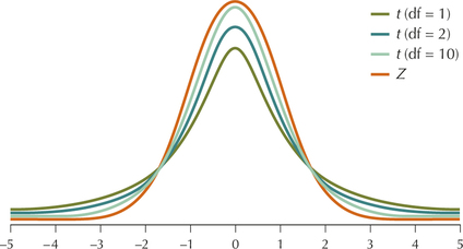
Figure 14 displays a comparison of some t curves with the Z curve. Note that there is only one Z distribution (or curve), but there is a different t curve for every different degrees of freedom (df), that is, for every different sample size. The degrees of freedom, df=n−1, determines the shape of the t distribution, just as the mean and variance uniquely determine the shape of the normal distribution. All t curves have several characteristics in common.
Characteristics of the t Distribution
- Centered at zero. The mean of t is zero, just as with Z.
- Symmetric about its mean zero, just as with Z.
- As the degrees of freedom decreases, the t curve gets flatter, and the area under the t curve decreases in the center and increases in the tails. That is, the t curve has heavier tails than the Z curve.
- As degrees of freedom increases toward infinity, the t curve approaches the Z curve, and the area under the t curve increases in the center and decreases in the tails.
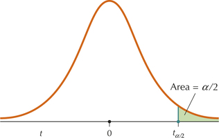
Similar to the definition of Zα/2 in Section 8.1, we can define tα/2 to be the value of the t distribution with area α/2 to the right of it, as seen in Figure 15. Table 1 in Section 8.1 provides the Zα/2 values for certain common confidence levels. Unfortunately, because there is a different t curve for each sample size, there are many possible tα/2 values. You will need to use the t table (Table D in the Appendix) to find the value of tα/2, as follows.
Procedure for Finding tα/2
- Step 1 Go across the row marked “Confidence level” in the t table (Table D in the Appendix) until you find the column with the desired confidence level at the top. The tα/2 value is in this column somewhere.
- Step 2 Go down the column until you see the correct number of degrees of freedom on the left. The number in that row and column is the desired value of tα/2.
EXAMPLE 12 Finding tα/2
Find the value of tα/2 that will produce a 95% confidence interval for μ if the sample size is n=20.
Solution
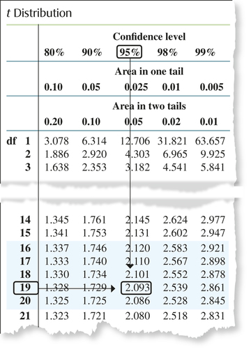
- Step 1 We go across the row labeled “Confidence level” in the t table (Figure 16) until we see the 95% confidence level. Our tα/2 is somewhere in this column.
- Step 2 The degrees of freedom are df=n−1=20−1=10. We go down the column until we see 19 on the left. The number in that row is our tα/2, 2.093.
Note: For the newer TI-84s
- Press 2nd DISTR and select 4:invT.
- Enter the area to the left of the t value, then comma, then df=n−1.
- Press ENTER.
For example, invT(0.975,19) gives 2.093024022. The TI-83 does not have this function.
NOW YOU CAN DO
Exercises 5–8.
YOUR TURN#7
Find the value of tα/2 that will produce a 90% confidence interval for μ if the sample size is n=20.
(The solution is shown in Appendix A.)
2 t Interval for the Population Mean
The t distribution provides the following confidence interval for the unknown population mean μ, called the t interval.
Note: Suppose that σ is unknown, and the population is either non-normal or of unknown distribution, and the sample size is not large. Then we should not use the t interval. Instead, we need to turn to nonparametric methods, for example, the sign interval or the Wilcoxon interval. (See Chapter 14: Nonparametric Statistics, available online.)
t Interval for μ
The t interval for μ may be constructed whenever either of the following conditions is met:
- The population is normal.
- The sample size is large (n≥30).
Suppose a random sample of size n is taken from a population with unknown mean μ and unknown standard deviation σ. A 100(1−α)% confidence interval for μ is given by the interval
lower bound=ˉx−tα/2(s/√n), upper bound=ˉx+tα/2(s/√n)
where ˉx is the sample mean, tα/2 is associated with the confidence level and n−1 degrees of freedom, and s is the sample standard deviation. The t interval may also be written as
ˉx±tα/2(s/√n)
and is denoted
(lower bound, upper bound)
EXAMPLE 13 Checking whether the conditions are met for the t interval for μ
Never assume normality unless it is indicated or evidence for it exists.
For each of the following, we are taking a random sample from a population with σ unknown. Determine whether the conditions are met for constructing the indicated t interval for μ. If not, explain why not.
- Confidence level 99%, n=16, ˉx=35, s=8
- Confidence level 95%, n=25, ˉx=42, s=10, normal population
Solution
- The sample size is not large (n is not≥ , and we are not told that the population is normal. Therefore, the conditions are not met for the interval for . It is not okay to construct the interval.
- Again the sample size is not large, but this time we are told that the population is normal. Thus, the conditions are met for the interval for . It is okay to construct the interval.
NOW YOU CAN DO
Exercises 9–12.
YOUR TURN#8
For each of the following, we are taking a random sample from a population with unknown. Determine whether the conditions are met for constructing the indicated interval for . If not, explain why not.
- Confidence level 95%, , ,
- Confidence level 95%, , ,
(The solutions are shown in Appendix A.)
EXAMPLE 14 Constructing a confidence interval for
cerealsodium
Research has shown that the amount of sodium consumed in food has been associated with hypertension (high blood pressure). The table provides a list of 16 breakfast cereals, along with their sodium contents, in milligrams per serving.
- Determine whether the conditions are met for constructing a interval for the population mean sodium content per serving for all breakfast cereals.
- Find the value of for 99% confidence and degrees of freedom .
- Construct a 99% confidence interval for the population mean sodium content.
- Interpret the meaning of this confidence interval.
| Cereal | Sodium (grams) |
Cereal | Sodium (grams) |
|---|---|---|---|
| Apple Jacks | 125 | Grape Nuts Flakes | 140 |
| Cap'n Crunch | 220 | Kix | 260 |
| Cinnamon Toast Crunch | 210 | Life | 150 |
| Corn Flakes | 290 | Lucky Charms | 180 |
| Count Chocula | 180 | Raisin Bran | 210 |
| Cream of Wheat | 80 | Rice Chex | 240 |
| Fruit Loops | 125 | Special K | 230 |
| Fruity Pebbles | 135 | Total Whole Grain | 200 |
Solution
- Figure 17 contains the normal probability plot for the data set. Though not perfect, all points lie within the bounds, indicating acceptable normality. Thus, we proceed to construct the 99% confidence interval.FIGURE 17 Normal probability plot for sodium in cereal.
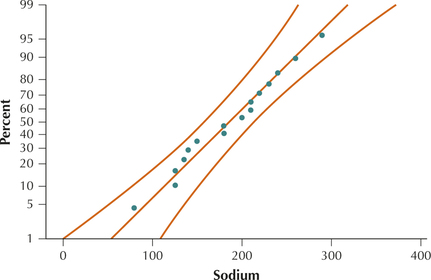
- The value of for 99% confidence and 15 degrees of freedom is 2.947.
A 99% confidence interval for is given by the interval
From the Minitab output in Figure 18, we have , , and . Substituting, we get:
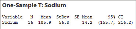
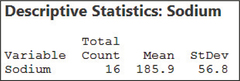 FIGURE 18 Minitab ouput.
- We are 99% confident that , the population mean sodium content per serving of all breakfast cereals, lies between 144.1 grams and 227.7 grams.
NOW YOU CAN DO
Exercises 13–28.
YOUR TURN#9
Find and interpret a 95% confidence interval for , which is the population mean sodium content per serving of all breakfast cereals.
(The solution is shown in Appendix A.)
Developing Your Statistical Sense
Intervals May Offer More Peace of Mind Than Intervals
In Example 14, if we had assumed that the population standard deviation was known , then the 99% interval for the population mean amount of sodium would have been
Note that this interval (149.3, 222.5) is only slightly more precise than the interval (144.1, 227.7). However, the interval depends on prior knowledge of the value of . If the value of is inaccurate, then the interval will be misleading and overly optimistic. With even moderate sample sizes, reporting the interval instead of the interval may offer peace of mind to the data analyst.
If the degrees of freedom needed to find do not appear in the df column of the table, a conservative solution is to take the next row with smaller df in the table. For example, if we have a data set such that , we find that is not in the table. Instead, we assign . (Even though 50 is closer, it will lead to an interval that overstates the precision in the data.) For , use the associated critical values, because the distribution approaches the distribution as gets very large.
Margin of Error
Recall that the margin of error for the interval equals . For the interval, because is unknown, the margin of error is given as follows.
Margin of Error for the Interval
The margin of error for a interval for can be interpreted as follows: “We can estimate to within units with confidence.”
EXAMPLE 15 Margin of error
Use the statistics observed in Example 14.
- Find the margin of error for the 99% confidence interval for mean sodium content per serving of all breakfast cereals.
- Interpret the margin of error.
Solution
From Example 14c, we have:
The margin of error for mean sodium content is 41.8 grams.
- We can estimate the population mean sodium content per serving of all breakfast cereals to within 41.8 grams with 99% confidence.
NOW YOU CAN DO
Exercises 29–40.
YOUR TURN#10
Find and interpret the margin of error for the 95% confidence interval for mean sodium content found in the Your Turn #9 after Example 14.
(The solution is shown in Appendix A.)
What Does the Margin of Error Mean?
The margin of error provides an indication of the accuracy of the confidence interval estimate for confidence level = 99%. That is, if we repeatedly take many samples of size 16 breakfast cereals, our sample mean will be within of the unknown population mean in 99% of those samples.
EXAMPLE 16 intervals for using technology
cerealsodium
For the breakfast cereal data in Example 14, construct a 99% confidence interval for the population mean sodium content, using the TI-83/84, Minitab, and SPSS.
Solution
We use the instructions provided in the Step-by-Step Technology Guide below. The sample size is not large (≤30), so it is necessary to check for normality. Figure 17 indicates acceptable normality.
The results for the TI-83/84 in Figure 19 display the 95% confidence interval for the population mean sodium content to be
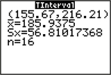
They also show the sample mean , the sample standard deviation , and the sample size .
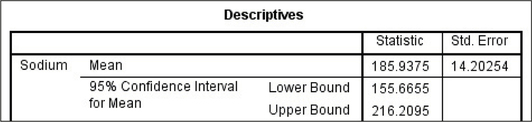
The Minitab results are shown in Figure 20, providing the sample size , the sample mean , the sample standard deviation , the standard error (SE mean) 14.2, and the 95% confidence interval (155.7, 216.2).
The SPSS results are shown in Figure 21, providing the sample mean , the standard error 14.20254, and the 95% confidence interval (155.6655, 216.2095).