8.1 Z Interval for the Population Mean
OBJECTIVES By the end of this section, I will be able to …
- Calculate a point estimate of the population mean.
- Calculate and interpret a Z interval for the population mean when the population is normal and when the sample size is large.
- Find ways to reduce the margin of error.
- Calculate the sample size needed to estimate the population mean.
1 Calculate a Point Estimate of the Population Mean
Recall from Section 1.2 that characteristics of a sample, such as the sample mean ˉx, are called statistics, whereas characteristics of a population, such as the population mean μ, are called parameters. Statistical inference consists of methods for estimating and drawing conclusions about parameters, based on the corresponding statistic. For example, we use the known value of ˉx to estimate the unknown value of μ.
Suppose a random sample of 30 male students at your school produced a sample mean height of ˉx=70 inches. We could then use this statistic ˉx=70 to infer that the population mean height μ of all male students at your school was close to 70 inches. This value of ˉx=70 is called a point estimate of the population mean μ.
Point estimation is the process of estimating unknown population parameters by known sample statistics. The value of each sample statistic used as an estimate is called a point estimate.
EXAMPLE 1 Calculating a point estimate

Farmers work hard to increase the yield of their acreage. Yield represents the number of bushels of a crop produced per acre. Suppose we are interested in estimating the population mean yield for winter wheat across all 50 states. Shown here is the mean July 2014 yield for a sample of five states, in bushels, as published by the U.S. Department of Agriculture (USDA).
- Find the sample mean yield ˉx.
- Express ˉx as the point estimate of μ, the unknown population mean winter wheat yield for all 50 states.
| State | Yield (bushels) |
|---|---|
| California | 85 |
| Georgia | 55 |
| Illinois | 67 |
| Ohio | 68 |
| Texas | 25 |
Solution
- The sample mean yield is calculated as
ˉx=∑xn=85+55+67+68+255=60
- The point estimate of μ, the unknown nationwide mean winter wheat yield for all 50 states, is 60 bushels per acre.
NOW YOU CAN DO
Exercises 11–14.
YOUR TURN#1
See Example 1. The USDA reports the yields for Colorado, Indiana, Maryland, Michigan, and Pennsylvania to be 36, 68, 65, 70, and 63 bushels, respectively.
- Find the sample mean yield ˉx.
- Express ˉx as the point estimate of μ, the unknown population mean winter wheat yield for all 50 states.
(The solutions are shown in Appendix A.)
However, because a sample is only a small subset of the population, generalizing from a sample to the population carries the risk that the point estimate may not be very accurate. For example, do you think that the population mean yield of winter wheat μ exactly equals our point estimate of 60 bushels per acre? It's not likely, because we learned in Example 1 of Chapter 7 (page 397) that different samples will produce different sample means, and thus different point estimates of μ. Our point estimate ˉx=60 may be close to μ or it may be far from μ. In other words, we have no measure of confidence that our particular point estimate is close to μ. There has to be a better way, and there is: confidence intervals, the subject of this chapter.
2 The Z Interval for the Population Mean
Although we cannot measure how confident we are of ˉx as a point estimate for μ, we can use the point estimate ˉx to find an interval that is likely to contain μ. Suppose we are interested in estimating the mean height of the students at your school. The students in your class are a sample of the population of students at your school, so we can calculate the sample mean height of the students in your class to be ˉx=67.5 inches (5 feet 7.5 inches tall).
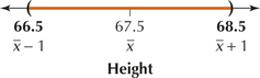
We are 90% confident that μ lies between 66.5 inches and 68.5 inches.
We may then use ˉx=67.5 inches as a point estimate of the unknown population mean height of all students at your school. However, this estimate is not likely to be exactly correct. To address this uncertainty in our estimate, we can use a range of heights instead, such as 67.5 inches, give or take an inch, which we write
67.5 inches ±1 inch
and would equal the interval
(66.5 inches, 68.5 inches).
The “1 inch” is called the margin of error. We might then say that we are 90% confident that the mean height of all students at our school lies in the
interval 67.5 inches ±1 inch (see the figure in the margin)
To increase the confidence in our estimate, we increase the margin of error, so that we might say we are 95% confident that the mean height of all students at our school lies in the interval 67.5 inches ±2 inches or the interval (65.5 inches, 69.5 inches). These two intervals are examples of what are called confidence intervals.
A confidence interval is an estimate of a parameter consisting of an interval of numbers based on a point estimate, together with a confidence level specifying the probability that the interval contains the parameter.
For example, our estimate that the mean height of all students at our school would lie in the interval (66.5 inches, 68.5 inches) was reported with confidence level 90%.
Confidence intervals are often reported in the format:
(lower bound, upper bound)
In the 90% confidence interval above, we have lower bound = 66.5 and upper bound = 68.5.
 Try not to confuse confidence interval with confidence level. A confidence interval is an interval of values on the number line. A confidence level is a percent, like 95%.
We use the α (alpha) notation here because it ties in with the notation we will need in Chapter 9, Hypothesis Testing.
A confidence level of 90% for a confidence interval means that, if we repeat the experiment 10 times, we would expect about 9 out of 10 times (90%) that the interval (lower bound, upper bound) will capture the population parameter.
Recall that, in previous chapters, we calculated probabilities for normal distributions using the standard normal Z. We can use Z to develop the formula for the Z confidence intervals for the population mean.
But before we do so, we need to define some notation.
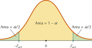
- Let α (alpha) be some small constant, usually (0<α≤0.10). The value of α is
α=1−confidence level
- Define Zα/2 to be the value of (standard normal) Z that has area α/2 to the right of it (see Figure 1). For example, for α=0.05, α/2=0.025 and Zα/2=Z0.025=1.96, as we know from Example 35 in Chapter 6 (page 362).
- The Z distribution is symmetric, so the area to the left of −Zα/2 is also α/2.
- Thus, area 1−α lies in the interval of values of Z between −Zα/2 and Zα/2. That is, the area 1−α lies in the interval −Zα/2<Z<Zα/2 (see Figure 1).
Next, we use the facts we learned in Chapter 7 about the sampling distribution of the sample mean to develop the formula for the confidence interval for the mean.
- Fact 1: μˉx=μ.
- Fact 2: σˉx=σ/√n (standard error of the mean).
- Fact 3: Sampling distribution is normal when the population is normal.
- Fact 4: Standardize ˉx to get
Z=ˉx−μσ/√n
Plugging this formula for Z back into the earlier inequality, −Zα/2<Z<Zα/2, gives
−Zα/2<ˉx−μσ/√n<Zα/2
We then use algebra to isolate μ as the middle term:
ˉx−Zα/2(σ/√n)<μ<ˉx+Zα/2(σ/√n)
Therefore, because areas represent probabilities, we can write
P(ˉx−Zα/2(σ/√n)<μ<ˉx+Zα/2(σ/√n))=1−α
The quantities on either side of μ in this inequality represent the lower bound and the upper bound for a 100(1−α)% confidence interval for μ. This confidence interval for μ is based on the standard normal Z distribution, so it is called the Z interval for the population mean μ.
To use the Z interval for μ, the value of σ must be known.
Z Interval for the Population Mean μ
The Z interval for μ may be constructed only when either of the following two conditions are met:
- The population is normally distributed, and the value of σ is known.
- The sample size is large (≥30), and the value of σ is known.
When a random sample of size n is taken from a population, a 100(1−α)% confidence interval for μ is given by
lower bound=ˉx−Zα/2(σ/√n)upper bound=ˉx+Zα/2(σ/√n)
where 1−α is the confidence level. The Z interval can also be written as
ˉx±Zα/2(σ/√n)
and is denoted
(lower bound, upper bound)
EXAMPLE 2 Determining whether the Z interval for μ may be used
For the following situations, state whether the Z confidence interval for the population mean μ may be used. Assume the population is normally distributed.
- The sample size is 30, but the value of σ is unknown.
- The sample size is 30, and the value of σ is known.
Solution
- Even though the population is normally distributed, the value of the population standard deviation σ is unknown, so the Z interval may not be used.
- Now the value of σ is known, and the population is normally distributed, so the Z interval may be used.
NOW YOU CAN DO
Exercises 15–20.
YOUR TURN#2
For the following situations, state whether the Z confidence interval for the population mean μ may be used:
- The population is not normally distributed, and the sample size is 10. The value of σ is known.
- The population is not normally distributed, and the sample size is 100. The value of σ is known.
(The solutions are shown in Appendix A.)
Two important results from Chapter 7 form the conditions that allow us to construct the Z interval for μ:
- The first condition comes from Fact 3 in Section 7.1: if the population is normal, then the sampling distribution of ˉx is also normal.
- The second condition is a result of the Central Limit Theorem for Means (from Section 7.1): if the sample size is large, then the sampling distribution of ˉx is approximately normal.
![]() The Normal Density Curve applet may be used to find Zα/2 critical values for confidence levels not listed in Table 1.
The Normal Density Curve applet may be used to find Zα/2 critical values for confidence levels not listed in Table 1.
Table 1 provides a listing of Zα/2 values for the most common confidence levels.
| Confidence level (1−α)100% | α | α/2 | Zα/2 |
| 100(1−0.20)%=80% | 0.20 | 0.10 | 1.28 |
| 100(1−0.10)%=90% | 0.10 | 0.05 | 1.645 |
| 100(1−0.05)%=95% | 0.05 | 0.025 | 1.96 |
| 100(1−0.01)%=99% | 0.01 | 0.005 | 2.576 |
EXAMPLE 3 Finding the value of Zα/2
For the following situations, find the value of Zα/2:
- Confidence level = 95%
- α=0.01
Solution
- From Table 1, we have Zα/2=1.96. We mentioned this case earlier (page 430), and in Example 35 of Chapter 6 (page 362).
- Table 1 gives us Zα/2=2.576.
NOW YOU CAN DO
Exercises 21–26.
YOUR TURN#3
For the following situations, find the value of Zα/2:
- Confidence level = 99%
- α/2=0.05
(The solutions are shown in Appendix A.)
EXAMPLE 4 Constructing a confidence interval for the mean of a normal population
The College Board reports that the scores on the 2014 SAT Math test were normally distributed. A sample of 25 SAT scores had a mean of ˉx=510. Assume that the population standard deviation of such scores is σ=118. Construct a 90% confidence interval for the population mean score on the 2014 SAT Math test.
Be careful! In order to use the Z interval for μ, the population standard deviation σ must be known, not just the sample standard deviation. If the word problem provides the sample standard deviation s but not the population standard deviation σ, then you cannot use the Z interval. You might be able to use the t confidence interval for μ (Section 8.2).
Solution
Because the population is normal and the population standard deviation σ is known, the requirements for the Z interval are met:
lower bound=ˉx−Zα/2(σ/√n)upper bound=ˉx+Zα/2(σ/√n)
We are given ˉx=510, σ=118, and n=25. From Table 1, we have Zα/2=1.645. Thus,
lower bound=510−1.645(118/√25)=471.2upper bound=510+1.645(118/√25)=548.8
We are 90% confident that the population mean score on the 2014 Mathematics SAT test lies between 471.2 and 548.8.
NOW YOU CAN DO
Exercises 27–30.
YOUR TURN#4
For the scenario in Example 4, construct a 95% confidence interval for the population mean score on the 2014 SAT Math test.
(The solution is shown in Appendix A.)
What Does This Confidence Interval Mean?
What does the 90% in the phrase 90% confidence interval mean? If we take sample after sample for a very long time, then in the long run, the proportion of intervals that will contain the population mean μ will equal 90%.
Interpreting Confidence Intervals
You may use the following generic interpretation for the confidence intervals that you construct: “We are 90% (or 95% or 99% and so on) confident that the population mean__________(for example, SAT Math score) lies between__________ (lower bound) and__________(upper bound).”
The Z interval for the population mean μ takes the form
point estimate± margin of error E
where the point estimate equals the sample mean ˉx and the margin of error E equals Zα/2(σ/√n).
The margin of error E is a measure of the precision of the confidence interval estimate. For the Z interval, the margin of error takes the form E=Zα/2(σ/√n). Smaller values of E indicate smaller margin of error, and therefore, greater precision.
Later in this section (page 437) we learn ways to reduce the margin of error.
For example, the confidence interval from Example 4 has the form
point estimate± margin of error E =ˉx±E =ˉx±Zα/2(σ/√n) =510±38.8
EXAMPLE 5 Constructing a Z interval for the population mean for a large sample size

 Motor Vehicle Fuel Efficiency
One of the variables in our case study is City MPG, which is the number of miles a vehicle can travel in city conditions on one gallon of gas. Because we have information on the entire population of 1141 vehicles, we know the population standard deviation σ=5.637 mpg. We obtained a sample of 100 vehicles and observed a sample mean city gas mileage of ˉx=20.71 mpg.
- Determine whether the requirements are met for constructing the Z interval for μ.
- Construct a 90% confidence interval for μ, the population mean City MPG for all vehicles.
- Interpret the confidence interval.
Note: As a check on your arithmetic, make sure that (lower bound+upper bound)2=ˉx.
In other words, the sample mean should lie exactly midway between the lower bound and the upper bound.
Solution
- We are not given any information about the distribution of the population, so we don't know if the population is normally distributed. However, the sample size n=100 is greater than 30, and the value of σ=5.637 is known; therefore, we can proceed to construct the confidence interval.
The formula for the confidence interval is given by
lower bound=ˉx−Zα/2(σ/√n)upper bound=ˉx+Zα/2(σ/√n)
We are given n=100, ˉx=20.71, and σ=5.637. For a confidence level of 90%, Table 1 provides the value of Zα/2=Z0.025=1.645. Plugging into the formula:
lower bound=20.71−1.645(5.637/√100)≈20.71−0.93=19.78upper bound=20.71+1.645(5.637/√100)≈20.71+0.93=21.64
- We are 90% confident that μ, the population mean City MPG for all motor vehicles, lies between 19.78 mpg and 21.64 mpg. (See Figure 2.)
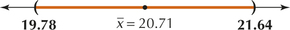 FIGURE 2 90% confidence interval for the population mean City MPG.
NOW YOU CAN DO
Exercises 31–34.
YOUR TURN#5
For the scenario in Example 5, construct a 99% confidence interval for μ, the population mean City MPG for all vehicles.
(The solution is shown in Appendix A.)
![]() The confidence Interval applet allows you to see for yourself how individual samples generate intervals that either do or do not contain the population mean.
The confidence Interval applet allows you to see for yourself how individual samples generate intervals that either do or do not contain the population mean.
Developing Your Statistical Sense
What Is Random Here?
It is important to understand that it is the interval that is random, not the population mean μ. The interval is formed by sample statistics such as ˉx, and for each different sample we get different values for the statistics. So the interval is random because it is constructed using ˉx, which is also random. The population mean μ, though usually unknown, is nevertheless constant.
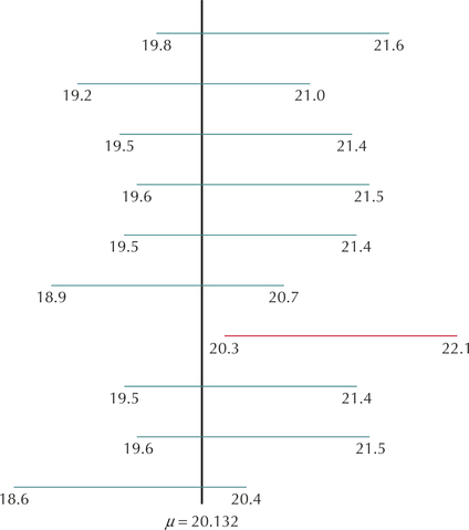
We generated 10 samples of size 100 vehicles from the Fuel Efficiency data set, and observed the City MPG of each vehicle. For each sample, a 90% Z confidence interval for the population mean City MPG was constructed. The results are shown in Figure 3. Note that, because we have the entire population of 1141 vehicles, we know the population mean City MPG is μ=20.132 mpg, which is also shown in Figure 3. Note that the confidence intervals are random, whereas μ is constant. The confidence intervals are random because they are based on the different values that the sample mean ˉx takes with each sample. The randomness involved in the sampling leads to the randomness of the values of ˉx. (This relates to what we learned in Chapter 7: the sample mean is a random variable that has its own distribution, the sampling distribution.)
Now, the confidence interval from our sample in Example 5 is shown as the first confidence interval, and is rounded to (19.8, 21.6). Note that this confidence interval happened to “capture” the population mean μ=20.132. However, one of the confidence intervals did not capture the population mean (the red one). It turns out that 9 out of 10 of the samples (90%) produced confidence intervals that contained μ. But it did not have to turn out this way. The 90% refers to the proportion of intervals that will contain μ after a great many samples are taken.
EXAMPLE 6 Z intervals for μ using technology
highwaympg16
Motor Vehicle Fuel Efficiency
Another of the variables in our case study is Highway MPG, which is the number of miles a vehicle can travel on a highway on one gallon of gas. We know the population standard deviation σ=6.326 mpg. The sample of 16 vehicles, shown here, has a sample mean highway gas mileage of ˉx=26.94 mpg.
| Vehicle | Highway MPG | Vehicle | Highway MPG |
|---|---|---|---|
| Honda CR-V | 30 | Subaru Impreza | 25 |
| Nissan Pathfinder | 26 | Ford Mustang | 26 |
| Acura MDX | 28 | Cadillac ATS | 31 |
| Porsche Cayenne | 29 | Chevrolet Camaro | 24 |
| Mercedes-Benz GLK 250 | 33 | Ford Taurus | 29 |
| Chevrolet Chevy SS | 21 | Ford Expedition | 20 |
| Dodge Charger | 27 | Lincoln MKT | 25 |
| Jeep Compass | 23 | BMW X1 | 34 |
- Determine whether the Z interval for μ may be applied.
- Use the TI-83/84, Minitab, and JMP to construct a 95% Z confidence interval for the population mean Highway MPG.
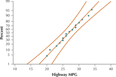
Solution
- The sample size n=16 is not large (≥30), so we need to check if the data follow a normal distribution. The normal probability plot of the data in Figure 4 supports the assumption of normality. Further, the population standard deviation is known. We may thus apply the n interval for μ.FIGURE 4 Normal probability plot of the Highway MPG data.
We shall use the instructions provided in the Step-by-Step Technology Guide at the end of this section (page 441). The results for the TI-83/84 in Figure 5 show that the 95% Z confidence interval for the population mean Highway MPG is
lower bound=23.838, upper bound=30.037
Figure 5 also shows the sample mean ˉx=26.9375, the sample standard deviation σ=3.991136012, and the sample size n=16.
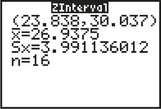 FIGURE 5 TI-83/84 results.
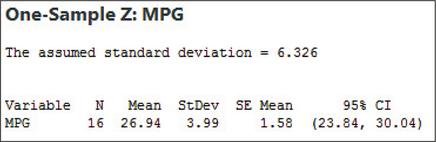
The Minitab results are provided in Figure 6. The “assumed standard deviation” is indicated to be σ=6.326. Then the sample size n=16, the sample mean ˉx=26.94, and the sample standard deviation s=3.99 are displayed. “SE Mean” refers to the standard error of the mean, but we don't need it here. Finally, the 95% confidence interval is given as (lower bound = 23.84, upper bound = 30.04).
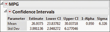
The JMP results are shown in Figure 7. The sample mean ˉx=26.9375 is shown in the first column, with the sample standard deviation s=3.991136 below it. The 95% confidence interval is given in the row labeled Mean, with lower bound = 23.84 (rounded) and upper bound = 30.04 (rounded).
3 Ways to Reduce the Margin of Error
Remember that the “±” notation always represents a pair of numbers.
Recall that the Z interval for μ takes the form
point estimate±margin of error=ˉx±E
where E=Zα/2(σ/√n). We interpret the margin of error E for a (1−α)100% confidence interval for μ as follows:
“We can estimate μ to within E units with (1−α)100% confidence.”
EXAMPLE 7 Finding and interpreting the margin of error
In Example 5, the Z interval for the population mean city gas mileage for all motor vehicles is:
lower bound=20.71−1.645(5.637/√100)≈20.71−0.93=19.78upper bound=20.71+1.645(5.637/√100)≈20.71+0.93=21.64
- Find the margin of error E.
- Express the confidence interval in the form “point estimate ± margin of error”
- Interpret the margin of error E.
Solution
- We find the margin of error as follows:
E=Zα/2(σ/√n)=1.645(5.637/√100)≈0.93 The point estimate is ˉx=20.71. Thus, the 95% confidence interval for the population mean city gas mileage for all motor vehicles takes the following form:
point estimate±margin of error =ˉx± Zα/2(σ/√n) =20.71±0.93
- We interpret the margin of error E by saying that we can estimate the population mean city gas mileage for all vehicles to within 0.93 mpg with 90% confidence.
NOW YOU CAN DO
Exercises 35–42.
Note: When it comes to the margin of error E, smaller is better!
Of course, we want our confidence interval estimates to be as precise as possible. Therefore, we want the margin of error to be as small as possible, which would in turn result in a tighter confidence interval. Tighter confidence intervals are better, because the likely maximum difference between the sample mean and the population mean is reduced.
So how do we reduce the size of the margin of error? Let's look at the margin of error for the Z interval:
E=Zα/2(σ/√n)
The population standard deviation σ is fixed, so only Zα/2 and n can vary. There are therefore two strategies for decreasing the margin of error:
- Decrease the confidence level, which would decrease the value of Zα/2 (see Table 1), and
- Increase the sample size n, because dividing by a larger √n will reduce E.
EXAMPLE 8 Decreasing the margin of error by decreasing the confidence level
For the confidence interval for the population mean city gas mileage in Example 5, suppose we reduce the confidence level from 90% to 80% and leave everything else unchanged. Find the new margin of error. Describe how the margin of error has changed.
Solution
From Example 5, we have the margin of error for the 90% confidence interval for μ as follows:
E=Zα/2(σ/√n)=1.645(5.637/√100)≈0.93
Decreasing the confidence level from 90% to 80% decreases Zα/2 from 1.645 to 1.28. This gives us the margin of error for the 90% confidence interval as:
E=Zα/2(σ/√n)=1.28(5.637/√100)≈0.72
Decreasing the confidence level from 90% to 80% decreases the margin of error from 0.93 mpg to 0.72 mpg.
Developing Your Statistical Sense
There's No Free Lunch
The margin of error in Example 8 is smaller than the one in Example 5, which is good because it gives a more precise estimate of μ. However, this smaller margin of error is due entirely to the decrease in the confidence level, which is not good. In statistical data analysis, there is rarely a free lunch. The trade-off here is that, while the margin of error went down, so did the confidence level, from 90% to 80%. On the other hand, confidence intervals that are too wide can be useless. For example, we can be 99.9999% confident that the population mean age of college students in Florida lies between 15 and 75 years old. But, so what? The interval is too wide to be of practical use. More useful would be a 95% confidence interval that the population mean age of college students in Florida lies between 20 and 27.
This leads us to Strategy 2 for reducing the margin of error: increase the sample size. The only way to have both high confidence and a tight interval is to boost the sample size.
EXAMPLE 9 Decreasing the margin of error by increasing the sample size
For the confidence interval for the population mean city gas mileage in Example 5, suppose the results were based on a sample of size n=400 instead of n=100. Leaving everything else unchanged, find the new margin of error, and describe how the margin of error has changed.
Solution
For n=400, the margin of error is
E=Zα/2(σ/√n)=1.645(5.637/√400)≈0.46
Increasing the sample size from n=100 to n=400 has decreased the margin of error from 0.93 mpg to 0.46 mpg.
“More data” is a familiar refrain in statistical analysis. Of course, increasing the sample size often raises pocketbook issues, because large samples can get very expensive (“We want a large-sample estimate of the amount of damage sustained by Corvettes hitting a wall at 90 mph”). Sometimes obtaining large samples is simply impossible. Suppose an astronomer has developed a new technique for predicting corona effects during solar eclipses; she will have to wait a while (say, a few hundred years) to build up a large sample. So, take samples as large as realistically possible to keep the width of the confidence interval as narrow as possible.
Increasingly, technology is being used to perform statistical analysis, including confidence intervals. Therefore, it is important to know how to read and interpret confidence intervals provided by software output. For instance, Example 10 shows how to calculate the margin of error E, when the software gives you only the lower bound and upper bound of the confidence interval.
EXAMPLE 10 Finding the margin of error, given the lower and upper bounds
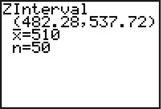
Figure 8 shows the results for a 95% Z confidence interval for μ, where μ represents the population mean score on the SAT Math test. Do the following:
- Report the confidence interval in the form “(lower bound, upper bound).”
- Interpret the confidence interval.
- Calculate the margin of error E for the confidence interval.
- Interpret the margin of error.
Solution
The TI-83/84 output gives us the following confidence interval:
(lower bound, upper bound)=(482.28,537.72)
We interpret this confidence interval as follows: We are 95% confident that the population mean score on the SAT Math test lies between 482.28 and 537.72.
Page 440Here, we show how to calculate the margin of error, given the lower bound and upper bound of the confidence interval. The confidence interval from (a) is illustrated in Figure 9.
FIGURE 9 Margin of error equals half the width of the confidence interval.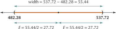
Now, the width of the margin of error is:
width=upper bound−lower bound
In Figure 9, the width of our confidence interval is:
width=537.72−482.28=55.44
Then, the margin of error is half this width, as shown in Figure 9. This gives us a margin of error of
E=margin of error=width/2=55.44/2=27.72
- We interpret the margin of error E by saying that we can estimate the population mean Math SAT score to within 27.72 points with 95% confidence.
NOW YOU CAN DO
Exercises 43–46.
In general, when the lower bound and upper bound of the confidence interval for μ have already been found, then the margin of error may be calculated as follows.
E=margin or error=(upper bound−lower bound)/2
4 Sample Size for Estimating the Population Mean
In general, more data implies more precise results. In fact, when samples are plentiful and cheap, arbitrarily precise confidence intervals with arbitrarily high confidence are possible simply by taking sufficiently large samples.
Therefore, the question arises: How large a sample size do I need to get a tight confidence interval with a high confidence level?
Note: We solve for n as follows:
E=(Zα/2)(σ/√n)
Multiply both sides by √n:
√n(E)=(Zα/2)σ
Divide both sides by E:
√n=((Zα/2)σE)
Square both sides to get the formula for n:
n=((Zα/2)σE)2
Sample Size for Estimating the Population Mean
The sample size for a Z interval that estimates the population mean μ to within a margin of error E with confidence 100(1−α)% is given by
n=((Zα/2)σE)2
where Zα/2 is the value associated with the desired confidence level (Table 1), E is the desired margin of error, and σ is the population standard deviation. By convention, whenever this formula yields a sample size with a decimal, always round up to the next whole number.
EXAMPLE 11 Sample size for estimating the population mean
We round up because (a) the sample size n must be a whole number and (b) rounding down will lead to a value of n with less than the desired confidence level.
Suppose we want to estimate to within $1000 the mean salary μ of all college graduates who were business majors. Assume σ=$5000. How many business majors would we sample to estimate the mean salary to within $1000 with 95% confidence?
Solution
“Within $1000” means that the desired margin of error E is $1000, and 1.96 is the Zα/2 value associated with 95% confidence. Substituting into the formula for the sample size, we get:
n=(1.96⋅50001000)2=96.04
Now, when finding the required sample size, if the formula results in a decimal, we always round up to the next whole number. Thus, we need a sample size of n=97 for a confidence level of 95%.
NOW YOU CAN DO
Exercises 47–54.
YOUR TURN#6
For the situation in Example 11, suppose we now needed our estimate to be within only $100 the mean salary μ. How many business majors would we sample to estimate the mean salary to within $100 with 95% confidence?
(The solution is shown in Appendix A.)