12.3 Randomized Block Design
OBJECTIVES By the end of this section, I will be able to …
- Explain the power of the randomized block design and perform a randomized block design ANOVA.
1 Randomized Block Design Explained and Performed
In the appropriate circumstances, we can use the randomized block design to improve the ability of the ANOVA to find significant differences among the treatment means. Suppose that a study was performed to determine whether significant differences existed among three types of educational methods: in-class learning, online learning, and the hybrid approach, which combines in-class and online learning. There were five courses taught in the study, and each course was taught using each method. For each course/method combination, the final exam average grade was calculated (see Table 6).
| Learning method | ||||
|---|---|---|---|---|
| In-class | Online | Hybrid | ||
| Course | Statistics | 75 | 70 | 69 |
| English | 80 | 77 | 82 | |
| Psychology | 72 | 69 | 72 | |
| Biology | 73 | 60 | 66 | |
| Communication | 88 | 82 | 85 | |
The researchers are not interested in the differences among the courses, only the differences in population mean performance among the learning methods. Thus, our factor of interest is the treatment variable learning methods, and our blocking factor is the variable course.
Another common term for the blocking factor is nuisance factor, which clearly indicates we are not interested in it.
A blocking factor, or block, is a variable that is not of primary interest to the researcher, but is included in the ANOVA in order to improve the ability of the ANOVA to find significant differences among the treatment means. In a randomized block design ANOVA, we test for differences among the treatment means, while accounting for the variability among the levels in the blocking factor.
Thus, in Table 6, the blocking factor course divides all the classes using a learning method into five blocks or courses.
We shall demonstrate the power of blocking by
- first performing a usual one-way ANOVA testing for differences among the learning methods, and then
- performing a randomized block design ANOVA, where we test for differences among the learning methods, while accounting for the variability among the courses (the blocks).
EXAMPLE 10 One-way ANOVA unable to find significance
finalexam
Use technology to perform a one-way ANOVA, using level of significance α=0.05, to determine whether the population mean test grades for the three learning methods are all the same.
Solution
If we ignore the blocking factor course, Table 6 becomes Table 7.
| Learning method | ||
|---|---|---|
| In-class | Online | Hybrid |
| 75 | 70 | 69 |
| 80 | 77 | 82 |
| 72 | 69 | 72 |
| 73 | 60 | 66 |
| 88 | 82 | 85 |
Figure 29 shows acceptable normality, and the largest of the standard deviations in the ANOVA output in Figure 30 and Figure 31 is not larger than twice the smallest.
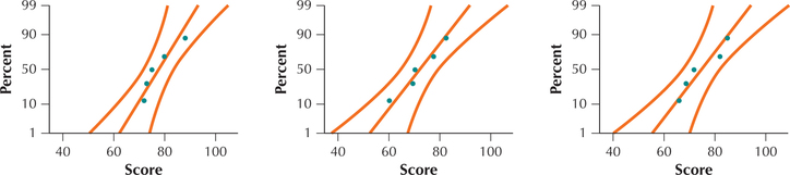
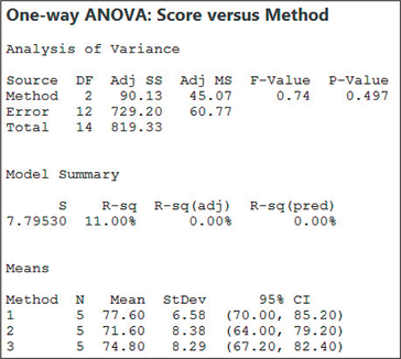
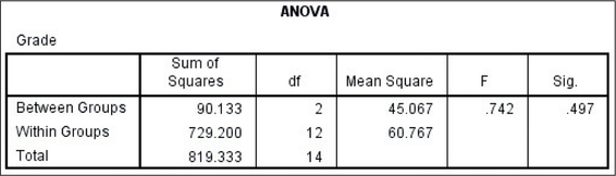
Thus, we may proceed with the ANOVA. The hypotheses are
HO:μIn-class=μOnline=μHybrid versus Ha:not all the population means are equal
Reject H0 if the p-value≤0.05.
The p-value from Figure 30 is 0.497, which is not ≤0.05; therefore, we do not reject H0. There is insufficient evidence at level of significance α=0.05 that the population mean test performance differs among the three learning methods.
Next, we use the randomized block design to account for the variability among the courses.
EXAMPLE 11 Randomized block design uncovers the significant differences among the learning methods
Note that the p-value for the blocking factor is approximately zero, which means that the blocking factor is significant. But in the randomized block design we are not interested in the significance of the blocking factor. If we are interested in a second factor, we use two-way ANOVA in Section 4.
Use technology and the randomized block design (RBD) to test for differences among the population mean test grades, at level of significance α=0.05.
Solution
We use the Step-by-Step Technology Guide at the end of this section to run this analysis in Minitab and SPSS. The hypotheses and the rejection rule are the same for RBD as they are for one-way ANOVA:
HO:μIn-class=μOnline=μHybrid versus Ha:not all the population means are equal
Reject H0 if the p-value≤0.05.
Figure 32 shows the Minitab output from the randomized block design, and Figure 33 shows the SPSS output. The factor of interest (that is, the treatment) is the learning method, whereas the blocking factor is the course. Note that there are two p-values, but we examine the p-value of the treatment only, not of the blocking factor.
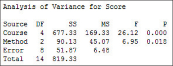
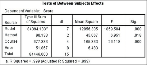
The p-value for the factor of interest from both Figure 32 and Figure 33 is 0.018, which is ≤0.05; therefore, we reject H0. There is evidence at level of significance α=0.05 that the population mean test grade differs among the three learning methods.
NOW YOU CAN DO
Exercises 5–10.
Developing Your Statistical Sense
How Does Blocking Work?
Why did the randomized block design succeed in rejecting the null hypothesis, when the usual one-way ANOVA failed? From Section 1, we know that the following relationship exists among the three sums of squares:
SST=SSTR+SSE
Now, the sum of squares error (SSE) includes all unexplained variability, including random variation as well as the variability among the courses themselves. For example, note from Table 6 that the three values from the communication courses are all larger than the three values from the statistics courses. This represents variability, and becomes part of SSE when we perform the usual ANOVA. In other words, the variability in the courses makes SSE larger than it should be.
Why is a large SSE bad? Recall our F statistic from the ANOVA table (Table 3, page 672):
F=MSTRMSE=MSTRSSE/df2
Recall that we reject H0 when the p-value is small. Also note that
- the p-value is small only when F is large (see Figure 34); and
- F is large when SSE is small.
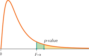 FIGURE 34 Larger F ↔ smaller p-value.
So we want to keep SSE small (as we would any type of error). The randomized block design reduces SSE by extracting the sum of squares blocks (SSB), which represents the variability among the groups in the blocking factor, such as the variability among the courses. This is done as follows. The SSE from the original one-way ANOVA is separated into the sum of two quantities:
SSEone-wayANOVA=SSB+SSERBD
Sums of squares are non-negative, so the new SSERBD from the RBD will probably be smaller than the original SSEone-way ANOVA, and thus F will become larger, leading to easier rejection of H0.
EXAMPLE 12 Demonstrating how RBd works
Demonstrate how randomized block design works, using the results from Examples 10 and 11.
Solution
Figure 30 from Example 10 provides us with
SSTR=90.133,SSEone-way ANOVA=729.2,and SST=819.333
The RBD from Example 11 (Figure 32) separates SSEone-way ANOVA into the sum of the following two quantities:
SSEone-wayANOVA=SSB+SSERBD=677.333+51.867=729.2
The new sum of squares error SSERBD is small enough that the resulting new F statistic is large, leading to a rejection of the null hypothesis.
Let k and b represent the number of treatments and the number of blocks, respectively. Then, the ANOVA table for the randomized block design is as shown in Table 8.
| Source | Sum of squares |
Degrees of freedom |
Mean square | F |
|---|---|---|---|---|
| Treatments | SSTR | k– | ||
| Blocks | SSB | |||
| Error | SSE | |||
| Total | SST |
Note the following facts about the ANOVA table for randomized block design:
- Notice that SSTR, its degrees of freedom , and MSTR are all the same quantities as in the one-way ANOVA table (Table 3) on page 672.
- is denoted simply as SSE.
- Quantities in the “Mean square” column equal the ratio of the quantities in the “Sum of squares” column divided by their respective degrees of freedom.
- We have , and the three degrees of freedom values sum to .
- We are not interested in the blocks and thus the mean square blocks MSB, so there is no statistic for blocks.
- In one-way ANOVA, the degrees of freedom for is . In RBD, this error degrees of freedom is partitioned into the degrees of freedom for SSB, , and the degrees of freedom for the new SSE, . An exercise in this section asks the student to show that these two degrees of freedom sum to .
NOW YOU CAN DO
Exercises 11–13.