14.5 Kruskal-Wallis Test
 This page includes Video Technology Manuals
OBJECTIVES By the end of this section, I will be able to …
- Perform the Kruskal-Wallis test for equal medians in three or more populations.
In Section 14.4, we learned the Wilcoxon rank sum test, which tests whether the population medians of two independent random samples are equal. Here, in Section 14.5, we extend this method from two populations to three or more populations.
1 Kruskal-Wallis Test for Equal Medians in Three or More Populations
The Kruskal-Wallis test is used to determine whether the population medians of three or more independent random samples are equal. In Chapter 12, we learned how to perform analysis of variance (ANOVA), which is a hypothesis test to determine if the population means of three or more populations are equal. However, ANOVA requires that each population be normally distributed. The Kruskal-Wallis test is less strict, in that it does not require that the populations be normally distributed. Thus, the Kruskal-Wallis test is more widely applicable than is ANOVA.
The Kruskal-Wallis test is a nonparametric hypothesis test in which the original data from three or more independent samples are transformed into their ranks. It tests whether the population medians are all equal.
To calculate the test statistic for the Kruskal-Wallis test, we temporarily combine all the data values from all the samples and find the ranks of the combined data values.
So far, this is exactly what we did for the Wilcoxon rank sum test, except that now we have k (three or more) samples instead of just two samples. Then the ranks are summed separately for each of the k samples.
- R1=the sum of the ranks for the first sample
- R2=the sum of the ranks for the second sample, and so on, until
⋮
- Rk=the sum of the ranks for thekth (last) sample
Let n1, n2, …, nk represent the sample sizes for samples 1,2,…,k, respectively. And let N represent the total number of data values in all the samples combined; that is, N=n1+n2+⋯+nk. To perform the Kruskal-Wallis test, each of the sample sizes n1,n2,…,nk must be at least 5. Then the Kruskal-Wallis test statistic is given by
χ2data=12N(N+1)(R21n1+R22n2+⋯+R2knk)−3(N+1)
When the conditions are met, χ2data follows a χ2 distribution with k−1 degrees of freedom.
EXAMPLE 16 Calculating the Kruskal-Wallis test statistic
citybusiness
The U.S. Small Business Administration publishes the number of small businesses in medium-size cities. We are interested in testing whether the population median number of small businesses per city is the same in Florida, North Carolina, and Texas. For the following independent random samples given in the table below, calculate the test statistic for the Kruskal-Wallis test, using these steps:
- Temporarily combine the three samples and arrange them in increasing order. Then rank the data values from smallest to largest. Resolve ties using the mean rank, as we have done in the previous sections.
- Calculate the sum of the ranks for each sample, R1, R2, and R3.
- Finally, calculate χ2data.
| Florida city | Number of small businesses |
North Carolina city |
Number of small businesses |
Texas city | Number of small businesses |
|---|---|---|---|---|---|
| Gainesville | 3,718 | Asheville | 4,883 | El Paso | 8,150 |
| Tallahassee | 4,948 | Wilmington | 5,825 | Lubbock | 4,403 |
| Daytona Beach | 9,489 | Greenville | 2, 153 | Killeen | 3,274 |
| Melbourne | 8,771 | Fayetteville | 3,424 | College Station | 2,276 |
| Sarasota | 13,729 | Rocky Mount | 2,108 | Laredo | 3,070 |
| Lakeland | 6,865 | Amarillo | 3,855 | ||
| Naples | 7,184 |
Solution
- The combined data, and their ranks, are shown here.
Combined data 2,108 2,153 2,276 3,070 3,274 3,424 3,718 3,855 4,403 Rank 1 2 3 4 5 6 7 8 9 Combined data 4,883 4,948 5,825 6,865 7,184 8,150 8,771 9,489 13,729 Rank 10 11 12 13 14 15 16 17 18 Page 14-38 The sum of the ranks for Florida is
R1=7+11+13+14+16+17+18=96
The sum of the ranks for North Carolina is
R2=1+2+6+10+12=31
The sum of the ranks for Texas is
R3=3+4+5+8+9+15=44
Also, there are 7 cities in the Florida sample, 5 cities in the North Carolina sample, and 6 cities in the Texas sample, so that n1=7, n2=5, and n3=6, and the total sample size is N=7+5+6=18.
Finally, the value of the test statistic is
χ2data=12N(N+1)(R21n1+R22n2+⋯+R2knk)−3(N+1)=1218(19)(9627+3125+4426)−3(19)≅7.261
Later, we will find out if this value for the test statistic warrants rejection of the null hypothesis. But first, we need to learn the hypotheses for the Kruskal-Wallis test.
NOW YOU CAN DO
Exercises 7–14.
Recall from Chapter 12 that the null hypothesis for ANOVA is that all population means are equal, and that the alternative hypothesis is that not all the population means are equal. The hypotheses for the Kruskal-Wallis test are the same, except that we are testing for medians instead of means.
Hypotheses for the Kruskal-Wallis Test
- H0:The population medians are all equal.
- Hα:Not all the population medians are equal.
Next, we will summarize the steps for performing the Kruskal-Wallis test for the equality of three or more population medians.
Kruskal-Wallis Test for k Independent Samples
The requirements are (a) there are k≥3 independent samples, each randomly selected, and (b) there are at least 5 data values in each sample. It is not required that the populations be normally distributed.
- Step 1 State the hypotheses.
- H0:The population medians are all equal.
- Ha:Not all the population medians are equal.
Step 2 Find the χ2 critical value χ2crit and state the rejection rule.
Use Appendix Table E. Select the column with “Area to the right of critical value” equal to the given level of significance α. The value of χ2crit is in the row with degrees of freedom k−1. The Kruskal-Wallis test is always a right-tailed test, so that the rejection rule is always to reject H0 if χ2data≥χ2crit.
Page 14-39Step 3 Find the value of the test statistic χ2data.
χ2data=12N(N+1)(R21n1+R22n2+⋯+R2knk)−3(N+1)
where
- R1=the sum of the ranks for the first sample
- R2=the sum of the ranks for the second sample, and so on, until
⋮
- Rk=the sum of the ranks for thekth (last) sample
and where n1,n2,…,nk represent the sample sizes for samples 1,2,…,k, respectively, and N=n1+n2+⋯+nk
- Step 4 state the conclusion and the interpretation. Compare the test statistic with the critical value, using the rejection rule.
EXAMPLE 17 Performing the Kruskal-Wallis test
Use the data in Example 16 to test whether the population median number of small businesses per city is the same in Florida, North Carolina, and Texas. Use the Kruskal-Wallis test with level of significance α=0.05.
Solution
Each sample is independent and randomly selected, and each sample has at least five data values. Thus, the conditions for the Kruskal-Wallis test are met, and we may proceed with the hypothesis test.
- Step 1 State the hypotheses.
- H0:The population median numbers of small businesses per city are all equal.
- Hα:Not all the population median numbers of small businesses per city are equal.
- Step 2 Find the χ2 critical value χ2crit and state the rejection rule. We have level of significance α=0.05. There are k=3 samples, so our degrees of freedom equals k−1=3−1=2. Using Appendix Table E, we select the column headed “0.05” and the row with degrees of freedom = 2. This gives us χ2crit=5.991 (see Figure 18). The rejection rule is to reject H0 if χ2data>5.991.
 FIGURE 18 Finding the χ2 critical value for the Kruskal-Wallis test.
 - Step 3 Find the value of the test statistic χ2data. From Example 16, we have χ2data≈7.261.
- Step 4 State the conclusion and the interpretation. Because 7.261≥5.991, we reject H0. Evidence exists that not all the population median numbers of small businesses per city are equal for Florida, North Carolina, and Texas.
NOW YOU CAN DO
Exercises 15–18.
EXAMPLE 18 Performing the Kruskal-Wallis test using technology

Recall the Chapter 12 Case Study, which investigated whether the amount of information a professor posts about himself or herself (that is, self-disclosure) on the online social network Facebook is related to student motivation.10 A professor constructed three different Facebook sites: one offering low self-disclosure, one offering medium self-disclosure, and one offering high self-disclosure. Study participants (students not enrolled in the professor's courses) were then randomly and independently assigned to access and browse one of the three Facebook sites, develop an impression of the professor, and complete the research questionnaire. Student motivation was measured using a set of 16 items, and the sum of the 16 items was calculated to form the total motivation score. Use technology and the Kruskal-Wallis test at level of significance α=0.01 to test whether the population median motivation scores are equal for the three types of Facebook pages (low, medium, and high self-disclosure). There were 43 students assigned to the low-disclosure page, 43 assigned to the medium-disclosure page, and 44 assigned to the high-disclosure page.
Solution
Each sample is independent and randomly selected, and there are at least five data values in each sample. Thus, the conditions for the Kruskal-Wallis test are met, and we may proceed with the hypothesis test.
- Step 1 State the hypotheses.
- H0:The population median motivation scores are all equal.
- Hα:Not all the population median motivation scores are equal.
- Step 2 Find the x2 critical value χ2crit and state the rejection rule. We have level of significance α=0.01. There are k=3 samples, so our degrees of freedom equals k−1=3−1=2. Using Appendix Table E, we find χ2crit=9.210. The rejection rule is to reject H0 if χ2data≥9.210.
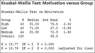
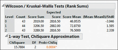
- Step 3 Find the value of the test statistic χ2data. We use the instructions in the Step-by-Step Technology Guide at the end of this section. Figure 19 shows the Minitab results from the Kruskal-Wallis test applied to the Facebook data. Figure 20 shows the output from the same test in JMP. Minitab denotes χ2data as “H” (use the one that is adjusted for ties). Thus, from Figure 19, χ2data=15.79.
 FIGURE 19 Minitab Kruskal-Wallis results.
 FIGURE 20 JMP Kruskal-Wallis results.
 - Step 4 State the conclusion and the interpretation. Because 15.29>9.210, we reject H0. There is evidence that not all the population median motivation scores are equal for the low-disclosure, medium-disclosure, and high-disclosure Facebook pages.