Section 4.3 Exercises
CLARIFYING THE CONCEPTS
Question 4.202
1. What does s measure? Would we want s to be large or small? Why? (p. 228)
4.3.1
The standard error of the estimate s is a measure of the size of the typical difference between the predicted value of y and the observed value of y.
Question 4.203
2. How does the least-squares criterion choose the “best” line to approximate the relationship between x and y? (p. 226)
Question 4.204
3. What does SSE measure? Would we want SSE to be large or small? Why? (p. 226)
4.3.3
SSE measures the prediction errors. SSE is the sum of the squared prediction errors. Since we want our prediction errors to be small, we want SSE to be as small as possible.
Question 4.205
4. What does SSR measure? Would we want SSR to be large or small? Why? (p. 230)
Question 4.206
5. What does SST measure? What statistic is it proportional to? (p. 229)
4.3.5
Measure of the variability in y. The variance s2 of the y's.
Question 4.207
6. What does it mean when r2 is close to 1? How about when it is close to 0? (p. 231)
Question 4.208
7. Do the values of x affect SST at all? (p. 229)
4.3.7
No
Question 4.209
8. Suppose we performed a regression analysis that resulted in r2=0.64. Without further information, would it be possible to calculate the correlation coefficient r? Explain. (p. 231)
Question 4.210
9. Suppose we performed a regression analysis on a data set that resulted in r2=0.64. Interpret this statistic in terms of the amount of variance in y explained by the linear relationship between x and y. (p. 231)
4.3.9
64% of the variability in the variable y is accounted for by the linear relationship between x and y.
Question 4.211
10. True or false: When the prediction errors are too small, the sum of squared error SSE can be negative. (p. 230)
PRACTICING THE TECHNIQUES
 CHECK IT OUT!
| To do | Check out | Topic |
|---|---|---|
| Exercises 11a–22a | Example 12 | SSE, the sum of squares error |
| Exercises 11b–22b | Example 13 | Standard error of the estimate, s |
| Exercises 11c–22c | Example 14 | SST, the total sum of squares |
| Exercises 11d–22d | Example 15 | SSR, the regression sum of squares |
| Exercises 11e–22e | Example 16 |
r2, the coefficient of determination |
| Exercises 11f–22f | Example 17 | Calculating r using r2 |
For Exercises 11–22, use the regression equations you calculated in Exercises 13–24 in Section 4.2. Do the following:
- Calculate the sum of squares error, SSE.
- Compute and interpret the standard error of the estimate, s.
- Calculate the total sum of squares, SST.
- Find the sum of squares regression, SSR.
- Calculate and interpret the coefficient of determination, r2.
- Use r2 to calculate the correlation coefficient, r.
Question 4.212
11.
| x | 10 | 20 | 30 | 40 |
| y | 2 | 5 | 9 | 12 |
4.3.11
(a) 0.2 (b) 0.316228. The typical difference between the predicted value of y and the actual observed value of y is 0.316228. (c) 58 (d) 57.8 (e) 0.9966. Therefore, 99.66% of the variability in y is accounted for by the linear relationship between y and x. (f) 0.9983
Question 4.213
12.
| x | 0 | 2 | 4 | 6 |
| y | 50 | 60 | 50 | 40 |
Question 4.214
13.
| x | −5 | −4 | −3 | −2 | −1 |
| y | 10 | 18 | 18 | 26 | 26 |
4.3.13
(a) 19.20 (b) 2.52982. The typical difference between the predicted value of y and the actual observed value of y is 2.52982. (c) 179.20 (d) 160 (e) 0.8929. Therefore, 89.29% of the variability in y is accounted for by the linear relationship between y and x. (f) 0.9449
Question 4.215
14.
| x | −3 | −1 | 1 | 3 | 5 |
| y | −25 | −35 | −40 | −45 | −50 |
Question 4.216
15.
| x | 5 | 10 | 15 | 20 | 25 | 30 |
| y | 7 | 8 | 8 | 8 | 7 | 8 |
4.3.15
(a) 1.27619 (b) 0.564843. The typical difference between the predicted value of y and the actual observed value of y is 0.564843. (c) 1.33333 (d) 0.05714 (e) 0.0429. Therefore, 4.29% of the variability in y is accounted for by the linear relationship between y and x. (f) 0.2071
Question 4.217
16.
| x | 6 | 7 | 8 | 9 | 11 | 13 |
| y | 9 | 9 | 9 | 9 | 9 | 9 |
Question 4.218
17.
| x | −70 | −60 | −50 | −40 | −30 | −20 | −10 | 0 |
| y | 5 | 10 | 15 | 20 | 20 | 15 | 10 | 5 |
4.3.17
(a) 250 (b) 6.45497. The typical difference between the predicted value of y and the actual observed value of y is 6.45497. (c) 250 (d) 0 (e) 0. Therefore, 0% of the variability in y is accounted for by the linear relationship between y and x. (f) 0
Question 4.219
18.
| x | −30 | −23 | −15 | −12 | −1 | 5 | 14 | 29 |
| y | 103 | 88 | 76 | 62 | 54 | 47 | 30 | 20 |
Question 4.220
19. The heights (in inches) and weights (in pounds) of a sample of five women are recorded.
| x=height | y=weight |
|---|---|
| 66 | 122 |
| 67 | 133 |
| 69 | 153 |
| 68 | 138 |
| 65 | 125 |
4.3.19
(a) 84.40 (b) 5.30409 pounds. The typical difference between the predicted value of y = weight and the actual observed value of y=weight is 5.30409 pounds. (c) 602.80 (d) 518.40 (e) 0.8600. Therefore, 86.00% of the variability in weight is accounted for by the linear relationship between y=weight and x = height. (f) 0.9274
Question 4.221
20. The number of days absent from a class, and the course grade.
| x= days absent | y= course grade |
|---|---|
| 0 | 95 |
| 2 | 90 |
| 4 | 85 |
| 6 | 70 |
| 8 | 60 |
Question 4.222
21. The number of hours spent on a repair job, and the cost of the repair.
| x= hours | y= cost |
|---|---|
| 2 | 120 |
| 3 | 180 |
| 5 | 230 |
| 8 | 350 |
| 10 | 380 |
4.3.21
(a) 1012 (b) 18.3662. The typical difference between the predicted value of y=cost and the actual observed value of y=cost is $18.3662. (c) 49080 (d) 48068 (e) 0.9794. Therefore, 97.94% of the variability in y=cost is accounted for by the linear relationship between y=cost and x = hours. (f) 0.9896
Question 4.223
22. The amount of rainfall at a baseball stadium (in inches), and attendance at the baseball game that day (in thousands).
| x= rain | y= attendance |
|---|---|
| 0.0 | 40 |
| 0.0 | 42 |
| 0.1 | 38 |
| 0.5 | 30 |
| 1.0 | 20 |
APPLYING THE CONCEPTS
For Exercises 23–37, follow these steps. You have already calculated the regression equation in Exercises 37–51 in Section 4.2. Do the following.
- Calculate the sum of squares error, SSE.
- Compute and interpret the standard error of the estimate, s.
- Calculate the total sum of squares, SST.
- Find the sum of squares regression, SSR.
- Calculate and interpret the coefficient of determination, r2.
- Use r2 to calculate and interpret the correlation coefficient, r.
Question 4.224
23. Video Game Sales. See Exercise 37 in Section 4.2.
4.3.23
(a) 0.59123 (b) 0.443933. The typical difference between the predicted number of total sales in millions of units and the actual observed number of total sales in millions of units is 0.443933 million units. (c) 1.30800 (d) 0.71677 (e) 0.5480. Therefore, 54.80% of the variability in total sales in millions of units is accounted for by the linear relationship between total sales in millions of units and weeks on top 30 list. (f) 0.7403. This value of r is close to the maximum value r=1. We would therefore say that the total sales in millions of units and weeks in the top 30 are positively correlated. As the number of weeks in the top 30 increases, the total sales in millions of units also tends to increase.
Question 4.225
24. Does It Pay to Stay in School? See Exercise 38 in Section 4.2.
Question 4.226
25. Darts and the Dow Jones. See Exercise 39 in Section 4.2.
4.3.25
(a) 2046 (b) 18.4665. The typical difference between the predicted value of the change in the stocks in the portfolio of stocks selected by the darts and the actual observed value of the change in the stocks in the portfolio of stocks selected by the darts is 18.4665. (c) 3659 (d) 1613 (e) 0.4408. Therefore, 44.08% of the variability in the change in the stocks in the portfolio of stocks selected by the darts is accounted for by the linear relationship between the change in the stocks in the portfolio of stocks selected by the darts and the change in the stocks in the DJIA. (f) 0.6639. This value of r is positive. We would therefore say that the change in the stocks in the portfolio of stocks selected by the darts and the change in the stocks in the DJIA are positively correlated. As the change in the stocks in the DJIA increases, the change in the stocks in the portfolio of stocks selected by the darts also tends to increase.
Question 4.227
26. Age and Height. See Exercise 40 in Section 4.2.
Question 4.228
27. Gardasil Shots and Age. See Exercise 41 in Section 4.2.
4.3.27
(a) 7.56875 (b) 0.972674 shot. The typical difference between the predicted number of shots and the actual observed number of shots is 0.972674. (c) 7.6 (d) 0.03125 (e) 0.0041. Therefore, 0.41% of the variability in the number of shots is accounted for by the linear relationship between the number of shots and age. (f) 0.0640. This value of r is close to r=0. We would therefore say that there is no linear relationship between the number of shots a child gets and the child's age.
Question 4.229
28. NCAA Power Ratings. See Exercise 42 in Section 4.2.
Question 4.230
29. Saturated Fat and Calories. See Exercise 43 in Section 4.2.
4.3.29
(a) 42.08 (b) 2.29340 grams. The typical difference between the predicted amount of saturated fat and the actual observed amount of saturated fat is 2.29340 grams. (c) 52.66 (d) 10.58 (e) 0.2009. Therefore, 20.09% of the variability in the amount of saturated fat is accounted for by the linear relationship between the amount of saturated fat and the calories per serving. (f) 0.4482. This value of r is positive. We would therefore say that the number of calories per serving and the number of grams of saturated fat per serving are positively correlated. As the number of calories in a serving of food increases, the number of grams of saturated fat also tends to increase.
Question 4.231
30. Engine Displacement and Gas Mileage. See Exercise 44 in Section 4.2.
Question 4.232
31. Completing College. See Exercise 45 in Section 4.2.
4.3.31
(a) 23.800 (b) 1.72483%. The typical difference between the predicted percent of a state's population that completes college and the actual observed percent of the state's population that completes college is 1.74283%. (c) 154.156 (d) 130.356 (e) 0.8456. Therefore, 84.56% of the variability in the percent of a state's population that completes college is accounted for by the linear relationship between the percent of a state's population that completes college and the percent of a state's population that attends college. (f) 0.9196.
This value of r is very close to the maximum value r=1. We would therefore say that the percent of a state's population that completes college and the percent of a state's population that attends college are positively correlated. As the percent of a state's population that attends college increases, the percent of a state's population that completes college tends to increase.
Question 4.233
32. Walking or Biking to Work. See Exercise 46 in Section 4.2.
Question 4.234
33. Teenage Birth Rate. See Exercise 47 in Section 4.2.
4.3.33
(a) 68.77 (b) 3.38560. The typical difference between the predicted teen birth rate and the actual observed teen birth rate is 3.38560. (c) 383.40 (d) 314.63 (e) 0.8206. Therefore, 82.06% of the variability in the teen birth rate is accounted for by the linear relationship between the teen birth rate and the overall birth rate. (f) 0.9059. This value of r is very close to the maximum value r=1. We would therefore say that the teen birth rate and the overall birth rate are positively correlated. As the overall birth rate increases, the teen birth rate also tends to increase.
Question 4.235
34. Brain and Body Weight. See Exercise 48 in Section 4.2.
Question 4.236
35. Consumer Sentiment. See Exercise 49 in Section 4.2.
4.3.35
(a) 358.82 (b) 5.99013. The typical difference between the predicted consumer sentiment for incomes $75,000 or higher and the actual observed consumer sentiment for incomes $75,000 or higher is 5.99013. (c) 440.01 (d) 81.19 (e) 0.1845. Therefore, 18.45% of the variability in the consumer sentiment for incomes $75,000 or higher is accounted for by the linear relationship between the consumer sentiment for incomes $75,000 or higher and the consumer sentiment for incomes under $75,000. (f) 0.4295. This value of r is positive. We would therefore say that the consumer sentiment for incomes $75,000 or higher and the consumer sentiment for incomes under $75,000 are positively correlated. As the consumer sentiment for incomes under $75,000 increases, the consumer sentiment for incomes $75,000 or higher also tends to increase.
Question 4.237
36. SAT Scores, by Foreign Language. See Exercise 50 in Section 4.2.
Question 4.238
37. Batting Average and Runs Scored. See Exercise 51 in Section 4.2.
4.3.37
(a) 530.02 (b) 8.13958. The typical difference between the predicted batting average of a player and the actual observed batting average of a player is 8.13958. (c) 560.50 (d) 30.48 (e) 0.0544. Therefore, 5.44% of the variability in the runs scored is accounted for by the linear relationship between the batting averages and the runs scored. (f) 0.2332. This value of r is close to the value r=0. We would therefore say that the batting averages and the runs scored have no linear relationship.
Regression in Accounting. Use the accounting data from Exercises 50–56 in Section 4.1 to answer Exercises 38–44.
Question 4.239
38. Compute a new variable, called net worth, which equals assets − liabilities.
Question 4.240
39. Perform a regression of current ratio on net worth. Interpret the coefficients.
4.3.39
ˆy=0.088x+1.03; b1=0.088 means that for each increase of $1 billion in the net worth of a company the current ratio increases by 0.088. b0=1.03 means that the predicted current ratio of a company with a net worth of x=$0 is 1.03.
Question 4.241
40. Regress current ratio on price-earnings ratio. Interpret the coefficients.
Question 4.242
41. What proportion of the variability in current ratio is accounted for by the following?
- Net worth
- Price-earnings ratio
4.3.41
(a) 10.79% (b) 5.97%
Question 4.243
42. How large is the typical residual when predicting current ratio using the following predictors?
- Net worth
- Price-earnings ratio
Question 4.244
43. Based on your answers to Exercises 41 and 42, which predictor, net worth or price-earnings ratio, is more useful for predicting current ratio?
4.3.43
Net worth
Question 4.245
44. Use the value of SST from Exercise 39 to calculate the variance of the current ratio data.
Best Places for Dating. Use the dating data from Exercises 57–59 in Section 4.1 to answer Exercises 45–48.
Question 4.246
45. Perform the following regressions:
- Overall dating score on percentage 18–24 years old
- Overall dating score on percentage 18–24 years old who are single
- Overall dating score versus online dating score
4.3.45
(a) y= overall dating score = 54.0 + 2.43 Percentage 18–24 years old (b) y= overall dating score = 134.5 – 0.646 Percentage 18–24 who are single (c) y= overall dating score = 67.1 + 0.194 Online dating score
Question 4.247
46. What proportion of the variability in overall dating score is accounted for by the following?
- Percentage 18–24 years old
- Percentage 18–24 years old who are single
- Online data score
Question 4.248
47. How large is the typical residual when predicting overall dating score using the following predictors?
- Percentage 18–24 years old
- Percentage 18–24 years old who are single
- Online data score
4.3.47
(a) 7.63309 (b) 7.50504 (c) 7.63561
Question 4.249
48. Based on your answers to Exercises 46 and 47, which predictor is most helpful for predicting overall dating score?
Virginia Weather. Use the data from Exercises 60–65 in Section 4.1 to answer Exercises 49–56.
Question 4.250
49. Perform a regression of heating degree-days on average January temperature.
4.3.49
Heating degree-days = 11264 – 198.1 Average January temperatures
Question 4.251
50. Interpret the slope of the regression line from Exercise 49.
Question 4.252
51. What is the size of the typical error in estimating heating degree-days using average January temperature?
4.3.51
164.753
Question 4.253
52. What proportion of the variability in heating degree-days is accounted for by average January temperature?
Question 4.254
53. Regress cooling degree-days on average July temperature.
4.3.53
Cooling degree-days = –8999 + 133.22 Average July temperatures
Question 4.255
54. How do we interpret the value of the slope of the regression equation from Exercise 53?
Question 4.256
55. Calculate the size of the typical residual when using average July temperature to predict cooling degree-days.
4.3.55
55.3145
Question 4.257
56. Find the proportion of the variability in cooling degree-days that is accounted for by the average July temperature.
Does It Pay to Stay in School? Refer to your work in Exercise 24 for Exercises 57 and 58.
Question 4.258
57. Answer the following:
- Which data value has the largest residual? Describe what is unusual about this observation.
- Suppose a public figure stated that 50% of the variability in the unemployment rate was due to competition from abroad. How would you use the regression results to respond to this claim?
- Suppose a politician claimed that using the years of education alone could allow us to predict the unemployment rate to within 1%. How would you use the regression results to respond to this claim?
- Suppose a newspaper claimed that each additional year of education brought down the unemployment rate by “more than 1%.” How would you use the regression results to either support or refute this claim?
4.3.57
(a) x=10 years of education; y=20.6= unemployment rate. It doesn't follow the trend of the higher the number of years of education, the lower the unemployment rate. (b) Since r2=0.6824, 68.24% of the variability in the variable y=unemployment rate is accounted for by the linear relationship between x=years of education and y=unemployment rate. Hence the statement is not true. (c) Since the absolute values of the residuals for 5, 10, and 16 years of education are more than 1%, this claim is not always true. (d) Since b1=−1.24, we can say that each additional year of education drops the predicted unemployment rate by 1.24%.
Question 4.259
 58. What if the unemployment rate for individuals with 5 years of education was not 16.8% but a much higher percentage? Describe how this would affect the slope and y intercept of the regression line. Explain your reasoning.
Question 4.260
59. Computational Formula for SST and SSR. The alternate computational formulas for finding SST and SSR are as follows:
SST=Σy2−(Σy)2/n SSR=[Σxy−(Σx)(Σy)/n]2Σx2−(Σx)2/n
Use the computational formulas to find SSR and SST for the memory score data on page 226. Assume we have the following summary statistics: Σx=40,Σy=150,Σxy=708,Σx2=214,Σy2=2478.
4.3.59
SST = 228, SSR = 216
BRINGING IT ALL TOGETHER
Fuel Economy. For Exercises 60–67, refer to the table of fuel economy data from Exercises 80–84 in Section 4.2. The predictor variable is x=engine size, expressed in liters; the response variable is y=combined (city/highway) gas mileage, expressed in miles per gallon (mpg).
Question 4.261
60. Calculating and interpreting the residuals and SSE and s.
- Compute the residual for each data value. Form a table similar to Table 7 of the residuals and squared residuals. Sum the squared residuals to get SSE.
- What does SSE measure? At this point, do we know whether SSE is large or small? Why or why not?
- Which vehicle has the largest absolute residual? Clearly explain why this vehicle is unusual.
Question 4.262
61. Calculating and Interpreting s.
- Calculate the value of s, the standard error of the estimate.
- Interpret the value of s, so that a nonstatistician could understand it.
4.3.61
(a) s=1.5887 (b) If we know car's engine size (x), then our estimate of the combined mpg will typically differ from the actual mpg by 1.5887 mpg.
Question 4.263
62. Computing and Interpreting SST, SSR, and r2.
- Calculate the sample variance of the y data, s2. Then use s2 to calculate SST.
- Use SSE and SST to find SSR. Explain clearly what it is that SSR is measuring.
- Calculate and interpret the coefficient of determination, r2.
Question 4.264
63. Correlation. Do the following:
- Use r2 and b1 to find the correlation coefficient, r.
- Interpret the correlation between engine size and combined mpg.
4.3.63
(a) r=−0.9585 (b) This value of r is very close to the minimum value r=−1. We would therefore say that the gas mileage and the engine displacement are negatively correlated. As the engine displacement of a car increases, the gas mileage of the car tends to decrease.
Question 4.265
64. What if we added one new vehicle to the data set, and its value was exactly (ˉx,ˉy)? How would this affect the slope and the y intercept?
Question 4.266
65. Refer to the previous exercise. What if we added an unknown amount to the engine size of the new vehicle? Describe how this change would affect the slope and the y intercept.
4.3.65
The slope would increase and the y intercept would decrease.
Question 4.267
66. Challenge Exercise. Suppose we increased the combined mpg for the Cadillac limousine, so that the slope of the regression line would be exactly zero. What would the combined mpg for the Cadillac limousine have to be to accomplish this?
Question 4.268
67. Challenge Exercise. Refer to the previous exercise. Describe how this change to the fuel economy of the Cadillac limousine would affect each of the following, and why: SSE, SSR, SST, s, r2, r.
4.3.67
Since b1=0, the regression equation is ˆy=ˉy=25.02. Thus ˆy−ˉy=0 for all of the ˆy−ˉy′s. Hence SSR = 0, so SSR would decrease. Since SST = SSR + SSE and SSR = 0, SSE = SST = 358.5622634, so both SSE and SST increase. Since the regression line doesn't include any information from the x-values, SSR = 0, r2=0, and r=0. Since SSR=0, r2=SSRSST, and r=√r2,r2=0 and r=0. Since s=√SSEn−2=6.6948 and SSE increases, s increases.
WORKING WITH LARGE DATA SETS
For Exercises 68–70, use technology and follow steps (a)–(e).
- Construct the scatterplot.
- Compute and interpret the regression equation.
- Calculate and interpret the coefficient of determination, r2.
- Compute and interpret s, the standard error of the estimate.
- Find r, using r2.
Question 4.269
darts
68. Open the darts data set, which we used for the Chapter 3 Case Study. Let x=the Dow Jones Industrial Average, and let y=the pros’ performance.
Question 4.270
nutrition
69. Open the nutrition data set. Let x=the amount of fat per gram, and let y=the number of calories per gram.
4.3.69
(a)
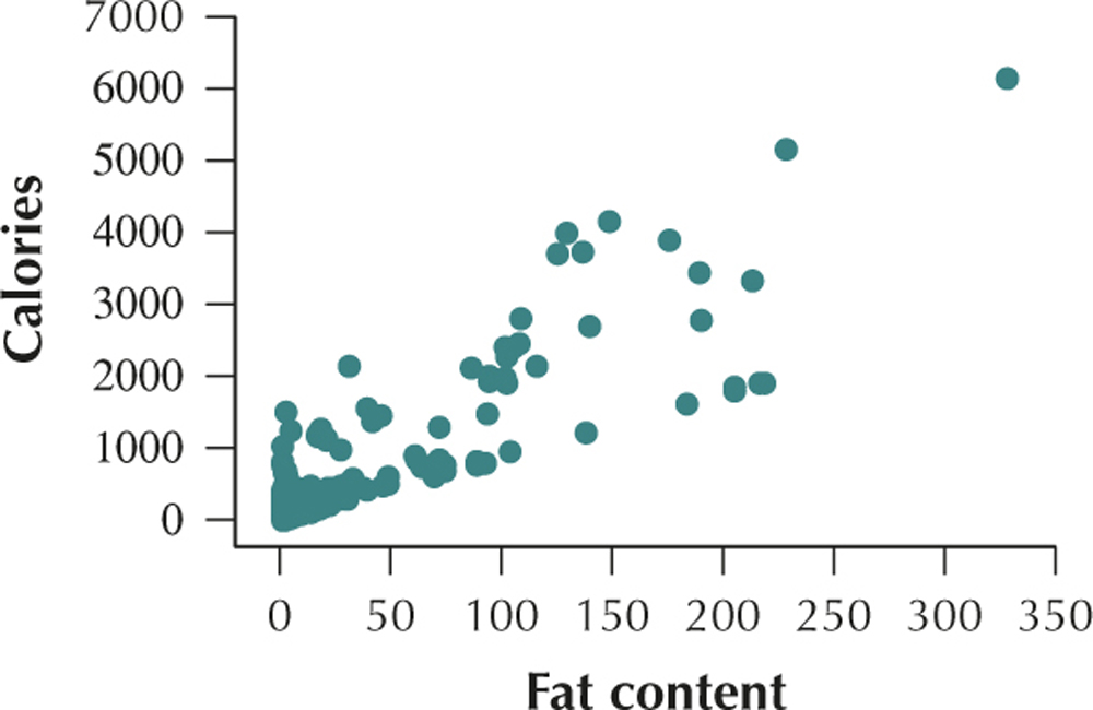
(b) ˆy=8.12x+1.28. The estimated calories per gram equals 8.12 times the amount of fat per gram, plus 1.28. (c) r2=0.736, so 73.6% of the variability in the number of calories per gram is accounted for by the linear relationship between calories per gram and fat per gram. (d) s=0.9944. The typical difference between the predicted number of calories per gram and the actual calories per gram is 0.9944. (e) r=√r2=√0.736=0.8579
Question 4.271
pulseandtemp
70. Open the pulse and temp data set. Let x=heart rate, and let y=body temperature.
CONSTRUCT YOUR OWN DATA SETS
Suppose we have a tiny data set with the following (x,y) pairs:
| x | y |
|---|---|
| 1 | ? |
| 2 | ? |
| 3 | ? |
For Exercises 71–75, create a set of y-values that would fulfill each specification.
Question 4.272
71. The slope of the line is positive.
4.3.71
Answers will vary.
Question 4.273
72. The slope of the line is negative.
Question 4.274
73. The slope of the line is 0.
4.3.73
Answers will vary.
Question 4.275
74. The slope of the line is equal to 2.
Question 4.276
75. The slope of the line is equal to −3.
4.3.75
Answers will vary.
![]() Use the Correlation and Regression applet for Exercises 76–78.
Use the Correlation and Regression applet for Exercises 76–78.
Question 4.277
76. In these applet exercises, use the “thermometer” above the graph (where it says “Sum of squares =”) to help find the least-squares regression line interactively.
- Select five points so that the correlation coefficient is about 0.8. Then select “Draw line.”
- Make your best guess about where the least-squares regression line should be, and draw the line there.
Question 4.278
77. The blue section of the thermometer is a measure of the sum of squares error, which is the total squared vertical distance from the data points to the actual regression line. Recall that the least-squares regression line minimizes this distance. The green section of the thermometer tells you how much “extra” squared error you get from using the line you constructed in Exercise 76(a).
- Adjust the line you drew in Exercise 76(a) by clicking and dragging on the points until the green section of the thermometer has disappeared.
- What does the disappearance of the green part tell you about the adjusted line you constructed?
- Will the line now coincide with the least-squares regression line?
4.3.77
(a) Answers will vary. (b) That your adjusted line matches the least squares regression line (c) Yes
Question 4.279
78. Verify that your adjusted line from Exercise 77 coincides with the least-squares regression line by selecting “Show least-squares line.”
WORKING WITH LARGE DATA SETS
 Chapter 4 Case Study: Measuring the Human Body. Open the data sets body_females and body_males. We shall apply what we have learned in this section regarding regression analysis to some of the measurements in these data sets. Use technology for Exercises 79–92.
  body_males
Question 4.280
body_females
body_males
79. For the regression of weight on height for females, find and interpret the standard error of the estimate, s.
4.3.79
19.1723 pounds. The typical difference between the predicted weight of a woman and the actual weight of a woman is 19.1723 pounds.
Question 4.281
body_females
body_males
80. For the regression of weight on height for females, calculate and interpret the coefficient of determination, r2
Question 4.282
body_females
body_males
81. Use r2 and the sign for the slope to compute the correlation coefficient for women’s heights and weights.
4.3.81
0.4303
Question 4.283
body_females
body_males
82. For the regression of weight on height for men, find and interpret the standard error of the estimate, s.
Question 4.284
body_females
body_males
83. For the regression of weight on height for males, calculate and interpret the coefficient of determination, r2.
4.3.83
0.2863. Therefore, 28.63% of the variability in men's weights is accounted for by the linear relationship between men's weights and men's heights.
Question 4.285
body_females
body_males
84. Use r2 and the sign for the slope to compute the correlation coefficient for men’s heights and weights.
Question 4.286
body_females
body_males
85. Discuss similarities and differences among your results for the females and the males, with respect to the regression of weight on height, as follows:
- The standard error of the estimate, s
- The coefficient of determination, r2.
4.3.85
(a) The values of s for men and women are both between 19 and 20 but are not the same. (b) The values of r2 for men and women are both low but the value of r2 for men is higher than the value of r2 for women.
Question 4.287
body_females
body_males
86. Perform a regression of bicep girth on thigh girth for females. State the regression equation in words. Interpret the slope and y intercept values.
Question 4.288
body_females
body_males
87. Find and interpret the standard error of the estimate for the regression of bicep girth on thigh girth for females.
4.3.87
1.79882 centimeters. The typical difference between the predicted bicep girth of a woman and the actual bicep girth of a woman is 1.79882 centimeters.
Question 4.289
body_females
body_males
88. For the regression of bicep girth on thigh girth for females, calculate and interpret the coefficient of determination, r2.
Question 4.290
body_females
body_males
89. Now run a regression of bicep girth on thigh girth for the men. State the regression equation in words. Interpret the slope and y intercept values.
4.3.89
Bicep girth_1 = 8.12 + 0.4651 Hip girth_1. ˆy=0.4651x+8.12. The predicted bicep girth of a man is 0.4651 times his thigh girth plus 8.12. b1=0.4651 means that for each increase of 1 centimeter in a man's thigh girth the predicted bicep girth increases by 0.4651 centimeter. b0=8.12 means that the predicted bicep girth of a man with a thigh girth of x=0 centimeters is 8.12 centimeters.
Question 4.291
body_females
body_males
90. Find and interpret the standard error of the estimate for the regression of bicep girth on thigh girth for males.
Question 4.292
body_females
body_males
91. For the regression of bicep girth on thigh girth for males, calculate and interpret the coefficient of determination, r2.
4.3.91
0.4388. Therefore, 43.88% of the variability in men's bicep girths is accounted for by the linear relationship between men's bicep girths and men's thigh girths.
Question 4.293
body_females
body_males
92. Discuss similarities and differences among your results for the females and the males, with respect to the regression of bicep girth on thigh girth, as follows:
- The slope
- The y intercept
- The standard error of the estimate, s
- The coefficient of determination, r2.