4.2 Introduction to Regression
 This page includes Video Technology Manuals
 This page includes Statistical Videos
OBJECTIVES By the end of this section, I will be able to …
- Calculate the value and understand the meaning of the slope and the y intercept of the regression line.
- Predict values of y for given values of x, and calculate the prediction error for a given prediction.
1 The Regression Line
In Section 4.1 we learned about the correlation coefficient. Here, in Section 4.2, we will learn how to approximate the linear relationship between two numerical variables using the regression line and the regression equation. For convenience, we repeat Table 3 here.
| City | x=low temperature | y=high temperature |
|---|---|---|
| Boston | 30 | 50 |
| Chicago | 35 | 55 |
| Philadelphia | 40 | 70 |
| Washington, DC | 45 | 65 |
| Dallas | 50 | 80 |
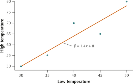
Consider again Figure 6 (page 193), the scatterplot of the high and low temperatures for five American cities, from Table 3. The data points generally seem to follow a roughly linear path. We may in fact draw a straight line from the lower left to the upper right to approximate this relatively linear path. Such a straight line, called a regression line, is shown in Figure 18.
highlowtemp
As you may recall from high school algebra, the equation of a straight line may be written as y=mx+b. We will write the equation of the regression line similarly as ˆy=b1x+b0.
Note: The “hat” over the y (pronounced “y-hat”) indicates that this is an estimate of y and not necessarily an actual value of y.
Equation of the Regression Line
The equation of the regression line that approximates the relationship between x and y is
ˆy=b1x+b0
where the regression coefficients are the slope, b1, and the y intercept, b0. Do not let ˆy and ˉy be confused. ˆy is the predicted value of y from the regression equation. ˉy represents the mean of the y-values in the data set. The equations of these coefficients are
b1=r⋅sysxb0=ˉy−(b1⋅ˉx)
where sx and sy represent the sample standard deviation for the x and y data, respectively.
An infinite number of different straight lines could approximate the relationship between high and low temperatures. Why did we choose this one? Because this is the least-squares regression line, which is the most widely used linear approximation for bivariate relationships. We will learn more about least squares in Section 4.3.
EXAMPLE 6 Calculating the regression coefficients b0 and b1
- Find the value of the regression coefficients b0 and b1 for the temperature data in Table 3.
- Write out the equation of the regression line for the temperature data.
- Clearly explain the meaning of the regression equation.
Solution
- We will outline the steps used in calculating the value of b1 using the temperature data.
- Step 1 Calculate the respective sample means ˉx and ˉy. We have already done this in Example 4 (page 193): ˉx=40 and ˉy=64.
- Step 2 Calculate the respective sample standard deviations sx and sy. We have already done this in Example 4: sx≈7.90569415 and sy≈11.93733639.
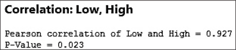
- Step 3 Find the correlation coefficient r. This was computed in Example 4: r≈0.92717265.
- Step 4 Combine the statistics from Steps 2 and 3 to calculate b1:
b1=r⋅sysx=0.92717265⋅11.937336397.90569415=1.4
- Step 5 Use the statistics from Steps 1–4 to calculate b0:
b0=ˉy−(b1⋅ˉx)=64−(1.4)(40)=8
- Thus, the equation of the regression line for the temperature data is
ˆy=1.4x+8
- Because y and x represent high and low temperatures, respectively, this regression equation is read as follows: “The estimated high temperature for an American city is 1.4 times the low temperature for that city plus 8 degrees Fahrenheit.”
NOW YOU CAN DO
Exercises 7–12 and 13a–24a.
YOUR TURN#6
 Measuring the Human Body
- Find the value of the regression coefficients b0 and b1 for the height and weight data from Table 2 (page 190).
- Write out the equation of the regression line for the height and weight data.
- Clearly explain the meaning of the regression equation.
(The solutions are shown in Appendix A.)
EXAMPLE 7 Interpreting the slope and the y intercept
Interpret the following values of the regression line we obtained in Example 6:
- The y intercept b0=8
- The slope b1=1.4
Solution
In statistics, we interpret the slope of the regression line as the estimated change in y per unit increase in x. In our temperature example, the units are degrees Fahrenheit, so we interpret our value b1=1.4 as follows:
“For each increase of 1°F in low temperature, the estimated high temperature increases by 1.4°F.”
The y intercept is interpreted as the estimated value of y when x equals zero. Here, we interpret our value b0=8 as follows:
“When the low temperature is 0°F, the estimated high temperature is 8°F.”
NOW YOU CAN DO
Exercises 13b–24b.
YOUR TURN#7
Measuring the Human Body
Interpret the following values of the regression line for the height and weight data from Table 2 (page 190):
- The y intercept b0
- The slope b1
(The solutions are shown in Appendix A.)
Recall from Section 4.1 that the correlation coefficient for the temperature data is r=0.9272. Is it a coincidence that both the slope and the correlation coefficient are positive? Not at all.
This relationship holds because b1=r⋅sysx and neither sy nor sx can be negative.
Relationship Between Slope and Correlation Coefficient
The slope b1 of the regression line and the correlation coefficient r always have the same sign.
- b1 is positive if and only if r is positive.
- b1 is negative if and only if r is negative.
Thus, when we found in Section 4.1 that the correlation coefficient between high and low temperatures was positive, we could have immediately concluded that the slope of the regression line was also positive
Other ways to describe regression include:
- “Perform a regression of the y variable versus the x variable.”
- “Regress the y variable on the x variable.”
Note that the first variable is always the y variable and the second variable is always the x variable. For example, in Example 7 we could write, “Perform a regression of high temperature against low temperature.”
EXAMPLE 8 Correlation and regression using technology
Use technology to find the correlation coefficient r and the regression coefficients b1 and b0 for the temperature data in Table 3 (page 193).
Solution
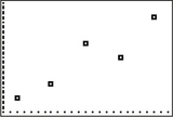
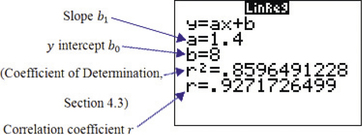
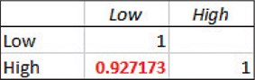
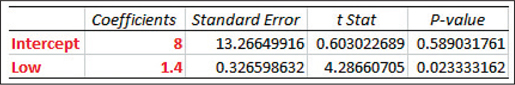
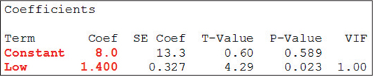
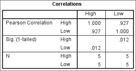
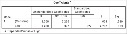
The instructions for using technology for correlation and regression are provided in the Step-by-Step Technology Guide at the end of this section (page 217). The TI-83/84 scatterplot is shown in Figure 19, and the TI-83/84 results are shown in Figure 20. (Note that the TI-83/84 indicates the slope b1 as a, and the y intercept b0 as b.) Figures 21 and 22 show the Excel results, with the y intercept (“Intercept”) and the slope (“Low”) highlighted. Figures 23 and 24 show excerpts from the Minitab results, with the y intercept (“Constant”) and the slope (“Low”) highlighted. Figures 25 and 26 show excerpts from the SPSS results.
2 Predictions and Prediction Error
We can use the regression equation to make estimates or predictions. For any particular value of x, the predicted value for y lies on the regression line.
EXAMPLE 9 Using the regression equation to make a prediction
Suppose we are moving to a city that has a low temperature of 40°F on this particular day. Use the regression equation in Example 6 to find the predicted high temperature for this city.
Solution
To generate an estimate of the high temperature, we plug in the value of 40°F for the x variable low:
ˆy=1.4(low)+8=1.4(40)+8=64
We would say, “The estimated high temperature for an American city with a low temperature of 40°F is 64°F.”
NOW YOU CAN DO
Exercises 25a–36a.
YOUR TURN#8
Measuring the Human Body
Use the regression equation you generated for the height and weight data in Table 2 to make a prediction of the weight for a female who is 63.5 inches tall.
(The solution is shown in Appendix A.)
Developing Your Statistical Sense
Actual Data versus Predicted (Estimated) Data
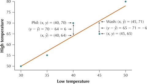
The city of Philadelphia in Table 3 has a low temperature of 40°F. The actual high temperature for Philadelphia is y=70°F, but our predicted high temperature is ˆy=64°F. Note the important difference in concept between y and ˆy. The actual high temperature in Philadelphia, y=70°F, is an established fact: real, observed data. On the other hand, our prediction, ˆy=64°F, is just an estimate based on a formula, the regression equation.
Prediction Error
Our prediction for Philadelphia’s high temperature was too low by
y−ˆy=70−64=6°
The difference is the vertical difference from the Philadelphia data point to the regression line. This difference is called the prediction error.
The prediction error or residual measures how far the predicted value of is from the actual value of observed in the data set. The prediction error may be positive or negative.
- Positive prediction error: The data value lies above the regression line, so the observed value of is greater than predicted for the given value of .
- Negative prediction error: The data value lies below the regression line, so the observed value of is lower than predicted for the given value of .
- Prediction error equal to zero: The data value lies directly on the regression line, so the observed value of is exactly equal to what is predicted for the given value of .
Prediction errors are also called estimation errors or residuals.
All values of (the predicted values of ) lie on the regression line.
EXAMPLE 10 Calculating and interpreting prediction errors (residuals)
Use the regression equation from Example 9 to calculate and interpret the prediction error (residual) for the following cities.
- Philadelphia: ,
- Washington, DC: ,
Solution
- The actual data point for Philadelphia is shown in the scatterplot in Figure 27 (denoted as “Phil”). In Example 9, we calculated the predicted high temperature for Philadelphia to be . In Figure 27, represents the -value of the point on the regression line where it intersects . That is, the actual high temperature lies directly above predicted temperature for low temperature .
- The actual high temperature in Washington that day was . Using the regression equation, the predicted high temperature is . So the prediction error is . The data point lies below the regression line, so that its actual high temperature of 65°F is lower than predicted given its low temperature of 45°F.

NOW YOU CAN DO
Exercises 25b–36b.
YOUR TURN#9
Measuring the Human Body
Recall the prediction you made in the previous Your Turn for the weight for a female who is 63.5 inches tall. Calculate the prediction error (residual) for this woman. Does her actual weight lie above or below the regression line?
(The solution is shown in Appendix A.)
Of course, we need not restrict our predictions to values of (low temperature) that are in our data set (but please see the warning on extrapolation below). For example, the estimated high temperature for a city in which is
Note that we cannot calculate the prediction error for this estimate because we do not have a city with a low temperature of 32°F to compare it to.

Extrapolation
The intercept is the estimated value for when equals zero. However, in many regression problems, a value of zero for the variable would not make sense. For example, a lot for sale of square feet does not make sense, so the intercept would not be meaningful. On the other hand, a value of zero for the low temperature does make sense. Therefore, we would be tempted to predict as the high temperature for a city with a low of zero degrees. However, is not within the range of the data set. Making predictions based on -values that are beyond the range of the -values in our data set is called extrapolation. It may be misleading and should be avoided.
Extrapolation consists of using the regression equation to make estimates or predictions based on -values that are outside the range of the -values in the data set.
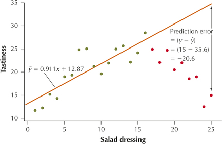
Extrapolation should be avoided, if possible, because the relationship between the variables may no longer be linear outside the range of . Consider Figure 28, which is the scatterplot of the tastiness versus amount of salad dressing we encountered in Section 4.1. Suppose we only had the data values shown in green, which show the tastiness tending to increase as the amount of salad dressing increases. These green data have -values ranging from to . The regression equation for these 16 points is . Now, suppose we made a prediction for , which lies outside the range of the -values. The predicted tastiness is a tastiness score of . However, the actual tastiness score for that much salad dressing is only 15, giving us a large prediction error of . This large prediction error is due to our extrapolation, where we made a prediction for for a value of for which we had no data, and which lay outside the range of the -values.
The further outside the range of , the more unreliable the prediction becomes.
EXAMPLE 11 Identifying when extrapolation occurs
Using the regression equation from Example 10, estimate the high temperature for the following low temperatures. If the estimate represents extrapolation, indicate so.
- 50°F
- 60°F
Solution
From Table 3, the smallest value of is 30°F and the largest is 50°F, so estimates for any value of between 30°F and 50°F, inclusive, would not represent extrapolation.
- . Because lies between 30°F and 50°F, inclusive, this estimate does not represent extrapolation.
- . Because does not lie between 30°F and 50°F, this estimate represents extrapolation.
NOW YOU CAN DO
Exercises 25c–36c.
YOUR TURN#10
Measuring the Human Body
Using the regression equation you constructed for the height and weight data from Table 2, estimate the weight for females with the following heights. If the estimate represents extrapolation, indicate so.
- 65 inches
- 70 inches
(The solutions are shown in Appendix A.)
![]() The Correlation and Regression applet allows you to insert your own data values and see how the regression line changes.
The Correlation and Regression applet allows you to insert your own data values and see how the regression line changes.