Section 6.4Exercises
CLARIFYING THE CONCEPTS
Question 6.215
1. For a continuous random variable X, why are we not interested in whether X equals some particular value? (p. 349)
6.4.1
The probability that X equals some particular value is zero.
Question 6.216
2. In the graph of a probability distribution, what is represented on the number line? (p. 349)
Question 6.217
3. How is probability represented in the graph of a continuous probability distribution? (p. 350)
6.4.3
Area under the normal distribution curve above an interval.
Question 6.218
4. What are the possible values for the mean of a normal distribution? For the standard deviation? (p. 352)
Question 6.219
5. True or false: The graph of the uniform distribution is always shaped like a square. (p. 350)
6.4.5
False
Question 6.220
6. For continuous probability distributions, what is the difference between P(X>1) and P(X≥1)? (p. 351)
Question 6.221
7. What is the value for the mean of the standard normal distribution? (p. 354)
6.4.7
0
Question 6.222
8. What is the value for the standard deviation of the standard normal distribution? (p. 354)
Question 6.223
9. True or false: The area under the Z curve to the right of Z=0 is 0.5. (p. 354)
6.4.9
True
Question 6.224
10. True or false: P(Z=0)=0. (p. 349)
PRACTICING THE TECHNIQUES
 CHECK IT OUT!
| To do | Check out | Topic |
|---|---|---|
| Exercises 11–20 |
Example 25 | Uniform probability distribution |
| Exercises 21–30 |
Example 26 | Normal distribution mean and standard deviation |
| Exercises 31–36 |
Example 27 | Properties of the normal curve |
| Exercises 37–44 |
Example 28 | Find the area to left of the Z -value |
| Exercises 45–48 |
Example 29 | Find the area to right of the Z -value |
| Exercises 49–58 |
Example 30 | Find the area between two Z -value |
| Exercises 59–70 |
Example 32 | Expressing areas under the standard normal curve as probabilities |
| Exercises 71–78 |
Example 33 | Finding the Z-value, given area to its left |
| Exercises 79–86 |
Example 34 | Finding the Z-value, given area to its right |
| Exercises 87–90 |
Example 35 | Find two Z-values that mark the boundaries of the middle 95% of the area |
For Exercises 11–16, assume that X is a uniform random variable, with left endpoint 0 and right endpoint 100. Find the following probabilities:
Question 6.225
11. P(50<X<100)
6.4.11
0.5
Question 6.226
12. P(50≤X≤100)
Question 6.227
13. P(25<X<90)
6.4.13
0.65
Question 6.228
14. P(15≤X≤35)
Question 6.229
15. P(24<X<25)
6.4.15
0.01
Question 6.230
16. P(25<X<25)
For Exercises 17–20, assume that X is a uniform random variable, with left endpoint −5 and right endpoint 5. Compute the following probabilities:
Question 6.231
17. P(0≤X≤5)
6.4.17
0.5
Question 6.232
18. P(−5≤X≤5)
Question 6.233
19. P(−5≤X≤−4)
6.4.19
0.1
Question 6.234
20. P(−1≤X≤5)
Question 6.235
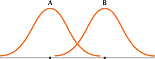
21. The two normal distributions in the accompanying figure have the same standard deviation of 5 but different means. Which normal distribution has mean 10 and which has mean 25? Explain how you know this.
6.4.21
A has mean 10; B has mean 25. The peak of a normal curve is at the mean; from the graphs we see that the mean of A is less than the mean of B.
Question 6.236
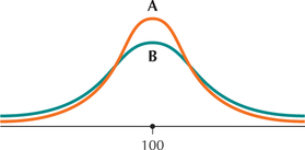
22. The two normal distributions in the figure below have the same mean of 100 but different standard deviations. Which normal distribution has standard deviation 3 and which has standard deviation 6? Explain how you know this.
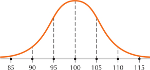
For Exercises 23–30, use the graph of the normal distribution to determine the mean and standard deviation. (Hint: The distance between dotted lines in the figures represents 1 standard deviation.)
Question 6.237
23.
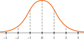
6.4.23
,
Question 6.238
24.
Question 6.239
25.
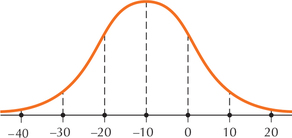
6.4.25
,
Question 6.240
26.
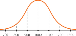
Question 6.241
27.
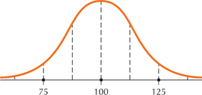
6.4.27
,
Question 6.242
28.
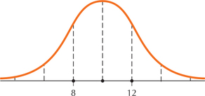
Question 6.243
29.
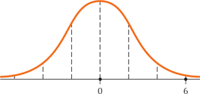
6.4.29
,
Question 6.244
30.
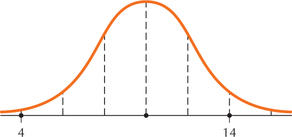
Use the normal distribution from Example 27 for Exercises 31–36. Birth weights are normally distributed with a mean weight of and a standard deviation of .
Question 6.245
31. What is the probability of a birth weight equal to 3285 grams?
6.4.31
0
Question 6.246
32. What is the probability of a birth weight more than 3285 grams?
Question 6.247
33. What is the probability of a birth weight of at least 3285 grams?
6.4.33
0.5
Question 6.248
34. What can we say about the area to the left of 3285 grams and the area to the right of 3285 grams?
Question 6.249
35. Is the area to the right of greater than or less than 0.5? How do you know this?
6.4.35
Less than 0.5. Since is greater than the mean of 3285 and the area to the right of is 0.5, the area to the right of is less than the area to the right of .
Question 6.250
36. Is the area to the left of greater than or less than 0.5? How do you know this?
For Exercises 37–58,
- draw the graph.
- find the area using the table or technology.
Find the area under the standard normal curve that lies to the left of the following:
Question 6.251
37.
6.4.37
(a)
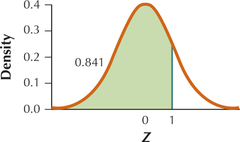
(b) 0.8143
Question 6.252
38.
Question 6.253
39.
6.4.39
(a)
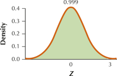
(b) 0.9987
Question 6.254
40.
Question 6.255
41.
6.4.41
(a)
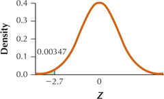
(b) 0.0035
Question 6.256
42.
Question 6.257
43.
6.4.43
(a)
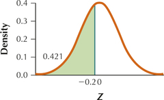
(b) 0.4207
Question 6.258
44.
Find the area under the standard normal curve that lies to the right of the following:
Question 6.259
45.
6.4.45
(a)
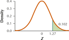
(b) 0.1020
Question 6.260
46.
Question 6.261
47.
6.4.47
(a)
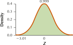
(b) 0.9987
Question 6.262
48.
Find the area under the standard normal curve that lies between the following:
Question 6.263
49. and
6.4.49
(a)
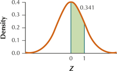
(b) 0.3413
Question 6.264
50. and
Question 6.265
51. and
6.4.51
(a)
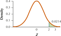
(b) 0.0214
Question 6.266
52. and
Question 6.267
53. and
6.4.53
(a)
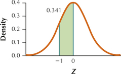
(b) 0.3413
Question 6.268
54. and
Question 6.269
55. and
6.4.55
(a)
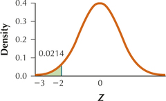
(b) 0.0214
Question 6.270
56. and
Question 6.271
57. and
6.4.57
(a)
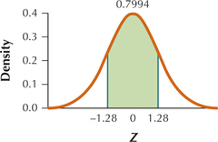
(b) 0.7994
Question 6.272
58. and
For Exercises 59–70, find the indicated probability for the standard normal .
- Draw the graph.
- Find the area using the table or technology.
Question 6.273
59.
6.4.59
(a)
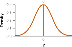
(b) 0
Question 6.274
60.
Question 6.275
61.
6.4.61
(a)
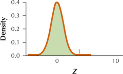
(b) 1
Question 6.276
62.
Question 6.277
63.
6.4.63
(a)
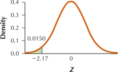
(b) 0.0150
Question 6.278
64.
Question 6.279
65.
6.4.65
(a)
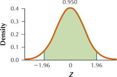
(b) 0.9500
Question 6.280
66.
Question 6.281
67.
6.4.67
(a)
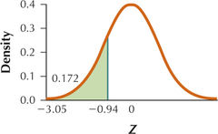
(b) 0.1725
Question 6.282
68.
Question 6.283
69.
6.4.69
(a)
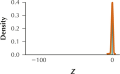
(b) 0.5000
Question 6.284
70.
For Exercises 71–78, find the -value with the following areas under the standard normal curve to its left. Draw the graph, and then find the -value.
Question 6.285
71. 0.3336
6.4.71
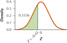
Question 6.286
72. 0.4602
Question 6.287
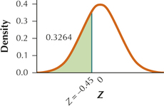
73. 0.3264
6.4.73
Question 6.288
74. 0.4247
Question 6.289
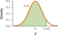
75. 0.95
6.4.75
1.65 (TI-83/84: 1.645)
Question 6.290
76. 0.975
Question 6.291
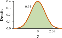
77. 0.98
6.4.77
2.05
Question 6.292
78. 0.99
For Exercises 79–86, find the -value with the following areas under the standard normal curve to its right. Draw the graph, and then find the -value.
Question 6.293
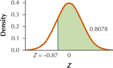
79. 0.8078
6.4.79
Question 6.294
80. 0.3085
Question 6.295
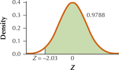
81. 0.9788
6.4.81
Question 6.296
82. 0.5120
Question 6.297
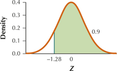
83. 0.90
6.4.83
𢄒1.28>
Question 6.298
84. 0.975
Question 6.299
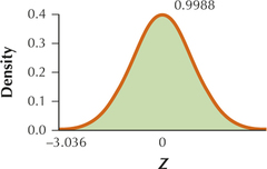
85. 0.9988
6.4.85
−3.036 (Using the table, both −3.03 and −3.04 have area to the left of them equal to 0.0012 and area to the right of them as 0.9988.)
Question 6.300
86. 0.9998
For Exercises 87–94, find the values of that mark the boundaries of the indicated areas.
Question 6.301
87. The middle 80%
6.4.87
−1.28 and 1.28
Question 6.302
88. The middle 95%
Question 6.303
89. The middle 98%
6.4.89
−2.33 and 2.33
Question 6.304
90. The middle 85%
Question 6.305
91. Find the 50th percentile of the distribution. (Hint: See margin note on page 360.)
6.4.91
Question 6.306
92. Find the 75th percentile of the distribution.
Question 6.307
93. Find the value of that is larger than 99.5% of all values of .
6.4.93
Question 6.308
94. Find the value of that is smaller than 99.5% of all values of .
APPLYING THE CONCEPTS
Question 6.309
95. Uniform Distribution: Web Page Loading Time.
Suppose that the Web page loading time for a particular home network is uniform, with left endpoint 1 second and right endpoint 5 seconds.
- What is the probability that a randomly selected Web page will take between 3 seconds and 4 seconds to load?
- Find the probability that a randomly selected Web page will take between 1 second and 2 seconds to load.
- How often does it take less than 1 second for a Web page to load?
- What is the probability that it takes exactly 2 seconds for a page to load? Explain.
6.4.95
(a) 0.25 (b) 0.25 (c) 0 (d) 0. Area underneath the curve for a single value of is the area of a line that is 0.
Question 6.310
96. Uniform Distribution: Random Number Generation.
Computers and calculators use the uniform distribution to generate random numbers. Suppose we have a calculator that randomly generates numbers between 0 and 1, so that they form a uniform distribution.
- What is the probability that the random number generated is less than 0.3?
- Find the probability that a random number is generated that is between 0.27 and 0.92.
What is the probability that a random number greater than 1 is generated?
Page 366- What is the probability that the exact number 0.5 is generated? Explain.
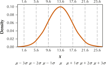
For Exercises 97–100, sketch the distribution, showing , and .
Question 6.311
97. Windy Frisco. The average wind speed in San Francisco in July is 13.6 miles per hour (mph), according to the U.S. National Oceanic and Atmospheric Administration. Suppose that the distribution of the wind speed in July in San Francisco is normal, with mean mph and standard deviation .
6.4.97
Question 6.312
98. Price of Crude Oil. The Organization of Petroleum Exporting States reports that the mean price for crude oil in July 2014 was $105.115 (one hundred five dollars, eleven and a half cents) per barrel. Assume the data is normal, with mean and standard deviation .
Question 6.313
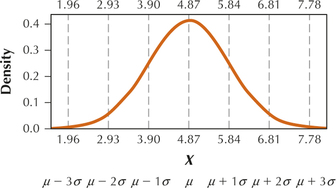
99. Hospital Patient Length of Stays. A study of Pennsylvania hospitals showed that the mean patient length of stay was 4.87 days, with a standard deviation of 0.97 day.16 Assume that the distribution of patient length of stays is normal.
6.4.99
Question 6.314
100. Facebook Friends. Statistica reported in 2014 that the mean number of Facebook friends for 18- to 24-year-olds was 649. Assume the distribution is normal, with friends and standard deviation friends.
Question 6.315
101. Percentiles of the Uniform Distribution. The th percentile of a continuous distribution is the value of that is greater than or equal to % of the values of . Find the following percentiles of the uniform distribution in Example 25:
- 95th
- 90th
- 97.5th
- 5th
- 10th
- 2.5th
6.4.101
(a) 9.5 minutes (b) 9 minutes (c) 9.75 minutes (d) 0.5 minute (e) 1 minute (f) 0.25 minute
Question 6.316
102. Mean of the Uniform Distribution. Explain two ways that you could find the mean of the uniform distribution.
- Use the balance point method.
- Find the median (50th percentile), and argue that, because the distribution is rectangle-shaped, the mean equals the median.
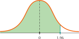
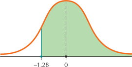
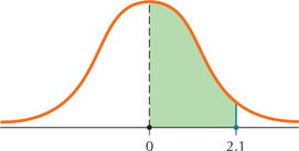
For Exercises 103–114, use the graph of the standard normal distribution to find the shaded area using the table or technology.
Question 6.317
103.
6.4.103
0.9750
Question 6.318
104.
Question 6.319
105.
6.4.105
0.4821
Question 6.320
106.
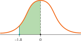
Question 6.321
107.
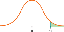
6.4.107
0.0179
Question 6.322
108.
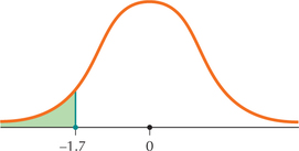
Question 6.323
109.
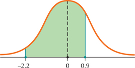
6.4.109
0.8020
Question 6.324
110.
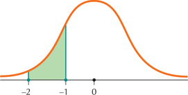
Question 6.325
111.
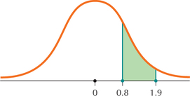
6.4.111
0.1832
Question 6.326
112.
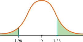
Question 6.327
113.
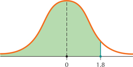
6.4.113
0.9641
Question 6.328
114.
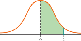
Question 6.329
115. Standardized Test Scores. Nicholas took a standardized test and was informed that the -value of his test score was 1.0. Find the percentages of test takers that Nicholas scored higher than.
6.4.115
0.8413
Question 6.330
116. Standardized Test Scores. Samantha's -value for her standardized test performance was 1.5. Calculate the proportion of test takers that Samantha scored higher than.
Question 6.331
117. High Jump. Brandon's score in the high jump at a track-and-field event showed that he was able to jump higher than 45% of the competitors. Find the -value for Brandon's high-jump score.
6.4.117
−0.13
Question 6.332
118. Body Temperature. The body temperatures of all the students in Kayla's class were measured. Kayla's body temperature was lower than 90% of her classmates. Find the -value corresponding to Kayla's body temperature.
Question 6.333
119. Checking the Empirical Rule. Check the accuracy of the Empirical Rule for . That is, find the area between and using the techniques of this section. Then compare your finding with the results for using the Empirical Rule.
6.4.119
The area between and is 0.9544. By the Empirical Rule, the area between and is about 0.95.
Question 6.334
120. Checking the Empirical Rule. Check the accuracy of the Empirical Rule for . That is, find the area between and using the techniques of this section. Then compare your finding with the results for using the Empirical Rule.
Question 6.335
121. Without Tables or Technology. Find the following areas without using the table or technology. The area to the left of is 0.0668.
- Find the area to the right of .
- Find the area to the right of .
- Find the area between and .
6.4.121
(a) 0.0668 (b) 0.9332 (c) 0.8664
Question 6.336
122. Without Tables or Technology. Find the following areas without using the table or technology. The area to the right of is 0.0035.
- Find the area to the left of .
- Find the area to the left of .
- Find the area between and .
Question 6.337
123. Values of That Mark the Middle 99%. Find the two values of that contain the middle 99% of the area under the standard normal curve.
6.4.123
and .
Question 6.338
124. Values of That Mark the Middle 90%. Find the two values of that contain the middle 90% of the area under the standard normal curve.
Question 6.339
125. Find the quartiles of the standard normal distribution. That is, find the 25th, 50th, and 75th percentiles of the standard normal distribution.
6.4.125
−0.67; 0; 0.67
BRINGING IT ALL TOGETHER
 Chapter 6 Case Study: SAT Scores and AP Exam Scores
The College Board reports that the population mean Critical Reading SAT score in 2013 was = 496, with a population standard deviation of , and that the scores followed a normal distribution. Use this information for Exercises 126–131.
Question 6.340
126. Draw the graph of this distribution. Mark the number line with the increments of and .
Question 6.341
127. Suppose a different exam had the following parameter values: and . Explain how the distribution graph would be similar and how it would be different from the graph in Exercise 126.
6.4.127
The peak would still be at but since the standard deviation is larger the curve would be flatter and more spread out.
Question 6.342
128. Suppose a different exam had the following parameter values: and . Explain how the distribution graph would be similar and would be different from the graph in Exercise 126.
Question 6.343
129. What can we say about and ? What property of the normal distribution allows us to say this?
6.4.129
They are both equal to 0.5. The property that the mean equals the median.
Question 6.344
130. Which of the following probabilities is larger: or ? How do you know this?
Question 6.345
131. Confirm your work from Exercise 130 as follows: The -value associated with is , and the -value associated with is . Find and . Does this confirm your work from Exercise 130?
6.4.131
and ; yes
