9 Hypothesis Testing

9.6 Chi-Square Test for the Population Standard Deviation

OBJECTIVES By the end of this section, I will be able to …

Perform the $χ^{2}$ test for $σ$ using the critical-value method.
Perform the $χ^{2}$ test for $σ$ using the $p$ -value method.
Use confidence intervals for $σ$ to perform two-tailed hypothesis tests about $σ$ .

1 $χ^{2}$ (Chi-Square) Test for $σ$ using the Critical-Value Method

In Section 8.4, we used the $χ^{2}$ distribution to help us construct confidence intervals for the population variance and standard deviation. Here, in Section 9.6, we will use the $χ^{2}$ distribution to perform hypothesis tests about the population standard deviation $σ$ . Why might we be interested in doing so? A pharmaceutical company that wants to ensure the safety of a particular new drug would perform statistical tests to make sure that the drug's effect was consistent and did not vary widely from patient to patient. The biostatisticians employed by the company would therefore perform a hypothesis test to make sure that the population standard deviation $σ$ was not too large.

Under the assumption that $H_{0} : σ = σ_{0}$ is true, the $χ^{2}$ statistic takes the following form:

$χ_{data}^{2} = \frac{(n - 1) s^{2}}{σ_{0}^{2}}$

Readers may want to review the characteristics of the $χ^{2}$ distribution in Section 8.4 on page 474.

For the hypothesis test about $s$ , our test statistic is called $χ_{data}^{2}$ because the values of $n - 1$ and $s^{2}$ come from the observed data. The test statistic $χ_{data}^{2}$ takes a moderate value when the value of $s^{2}$ is moderate, assuming $H_{0}$ is true, and $χ_{data}^{2}$ takes an extreme value when the value of $s^{2}$ is extreme, assuming $H_{0}$ is true. This leads us to the following.

The essential idea About Hypothesis testing for the Standard Deviation

When the observed value of $χ_{data}^{2}$ is unusual or extreme on the assumption that $H_{0}$ is true, we should reject $H_{0}$ . Otherwise, there is insufficient evidence against $H_{0}$ , and we should not reject $H_{0}$ .

The remainder of Section 9.6 explains the details of implementing hypothesis testing for the standard deviation. The $χ^{2}$ test for $σ$ may be performed using the $p$ -value method or the critical-value method. We begin with the critical-value method.

$χ^{2}$ Test for $σ$ : Critical-Value Method

This hypothesis test is valid only if we have a random sample from a normal population.

Step 1 State the hypotheses.

Use one of the forms in Table 13. State the meaning of $σ$ .
Step 2 Find the $χ^{2}$ critical value or values and state the rejection rule.

Use Table 13.
Step 3 Calculate $χ_{data}^{2}$ .

Either use technology to find the value of the test statistic $χ_{data}^{2}$ or calculate the value of $χ_{data}^{2}$ as follows:

Page 557

$χ_{data}^{2} = \frac{(n - 1) s^{2}}{σ_{0}^{2}}$

which follows a $χ^{2}$ distribution with $n - 1$ degrees of freedom, and where $s^{2}$ represents the sample variance.
Step 4 State the conclusion and the interpretation.

If $χ_{data}^{2}$ falls in the critical region, then reject $H_{0}$ . Otherwise do not reject $H_{0}$ . Interpret your conclusion so that a nonspecialist can understand.

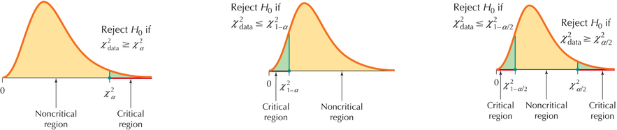
The $χ^{2}$ critical values in the right-tailed, left-tailed, or two-tailed tests use the following notations: $χ_{α}^{2}$ , $χ_{1 - α}^{2}$ , $χ_{α / 2}^{2}$ , and $χ_{1 - α / 2}^{2}$ (see Table 13). In each case, the subscript indicates the area to the right of the $χ^{2}$ critical value. Find these values just as you did in Section 8.4, using either technology or Table E, Chi-Square ( $χ^{2}$ ) Distribution, in the Appendix.

Table 9.41: Table 13 Critical values and rejection rules for the

$χ^{2}$ test for

$σ$

Right-tailed test	Left-tailed test	Two-tailed test
$\begin{array}{l} H_{0} : σ = σ_{0} \\ H_{a} : σ > σ_{0} \end{array}$	$\begin{array}{l} H_{0} : σ = σ_{0} \\ H_{a} : σ < σ_{0} \end{array}$	$\begin{array}{l} H_{0} : σ = σ_{0} \\ H_{a} : σ \neq σ_{0} \end{array}$
$\begin{array}{l} Critical value : X_{α}^{2} \\ Reject H_{0} if X_{data}^{2} \geq X_{α}^{2} \\ level of significance α \end{array}$	$\begin{array}{c} Critical value : X_{1 - α}^{2} \\ Reject H_{0} if X_{data}^{2} \leq X_{1 - α}^{2} \\ level of significance α \end{array}$	$\begin{array}{c} Critical values : X_{α / 2}^{2} and X_{1 - α / 2}^{2} \\ Reject H_{0} if X_{data}^{2} \geq X_{α / 2}^{2} \\ or if X_{data}^{2} \leq X_{1 - α / 2}^{2} \\ level of significance α \end{array}$

EXAMPLE 31 $χ^{2}$ test for $σ$ using the critical-value method

carbonemissions8

State	Carbon emissions (millions of metric tons)
Florida	230.98
Kentucky	148.36
Missouri	135.54
New Hampshire	16.41
New Mexico	56.60
New York	166.32
Tennessee	105.73
Virginia	99.86

Table 9.42: Carbon emissions

The table contains the carbon emissions from all sources for a random sample of eight states. Test whether the population standard deviation $σ$ of carbon emissions differs from 60 million metric tons, using level of significance $α = 0.05$ .

Page 558

Solution

The normal probability plot indicates acceptable normality.

Step 1 State the hypotheses.

The phrase “differs from” indicates that we have a two-tailed test. The value $σ_{0} = 60$ answers the question “Differs from what?” (Note that $σ_{0}$ is 60, and not 60,000,000 because the data are expressed in millions.) Thus, we have our hypotheses:

$\begin{array}{l} H_{0} : σ = 60 & versus & H_{a} : σ \neq 60 \end{array}$

where $σ$ represents the population standard deviation of carbon emissions in millions of metric tons.
Step 2 Find the $χ^{2}$ critical values and state the rejection rule.

We have $n = 8$ , so $degrees of freedom = n - 1 = 7$ . Because $α$ is given as 0.05, $α / 2 = 0.025$ and $1 - α / 2 = 0.975$ . Then, from the $χ^{2}$ table (Appendix Table E), we have $χ_{α / 2}^{2} = χ_{0.025}^{2} = 16.013$ , and $χ_{1 - α / 2}^{2} = χ_{0.975}^{2} = 1.690$ . We will reject $H_{0}$ if $χ_{data}^{2}$ is either $\geq χ_{α / 2}^{2} = 16.013$ or $\leq χ_{1 - α / 2}^{2} = 1.690$ .
Step 3 Find $χ_{data}^{2}$ .

The descriptive statistics in Figure 43 tell us that the sample variance is $s^{2} = 4409.7 million metric tons$ , squared.

FIGURE 43 Descriptive statistics from Minitab.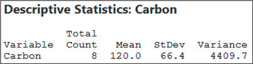

Thus, our test statistic is:

$χ_{data}^{2} = \frac{(n - 1) s^{2}}{σ_{0}^{2}} = \frac{(8 - 1) (4409.7)}{60^{2}} \approx 8.57$
Step 4 State the conclusion and the interpretation.

In Step 2, we said that we would reject $H_{0}$ if $χ_{data}^{2}$ was either $\geq 16.013 or \leq 1 .690$ . Because $χ_{data}^{2} = 8.57$ is neither $\geq 16.013 nor \leq 1.690$ (see Figure 44), we do not reject $H_{0}$ . There is insufficient evidence at level of significance $α = 0.05$ that the population standard deviation of the state carbon emissions differs from 60 million.

Page 559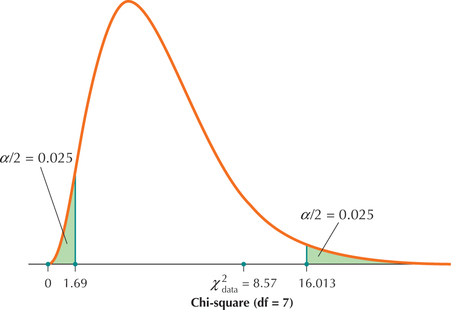

FIGURE 44 $χ_{data}^{2} = 8.57$ does not fall in critical region, so do not reject $H_{0}$ .

NOW YOU CAN DO

Exercises 7–12.

2 $χ^{2}$ Test for $σ$ Using the $p$ -Value Method

We may also use the $p$ -value method to perform the $χ^{2}$ test for $σ$ .

$χ^{2}$ test for $σ$ : $p$ -value Method

This hypothesis test is valid only if we have a random sample from a normal population.

Step 1 State the hypotheses and the rejection rule.

Use one of the forms in Table 14. State the rejection rule as “Reject $H_{0}$ when the $p-value \leq α$ .” State the meaning of $σ$ .
Step 2 Calculate $χ_{data}^{2}$ .

Either use technology to find the value of the test statistic $χ_{data}^{2}$ or calculate the value of $χ_{data}^{2}$ as follows:

$χ_{data}^{2} = \frac{(n - 1) s^{2}}{σ_{0}^{2}}$

which follows a $χ^{2}$ distribution with $n - 1$ degrees of freedom, and where $s^{2}$ represents the sample variance.
Step 3 Find the $p$ -value.

Use Table 14.
Step 4 State the conclusion and the interpretation.

If the $p-value \leq α$ , then reject $H_{0}$ . Otherwise, do not reject $H_{0}$ . Interpret your conclusion so that a nonspecialist can understand.

Table 9.43: Table 14

$p$ -Value method for the

$χ^{2}$ test for

$σ$

$\begin{array}{l} H_{0} : σ = σ_{0} \\ H_{a} : σ > σ_{0} \end{array}$

$\begin{array}{l} H_{0} : σ = σ_{0} \\ H_{a} : σ < σ_{0} \end{array}$

$\begin{array}{l} H_{0} : σ = σ_{0} \\ H_{a} : σ \neq σ_{0} \end{array}$

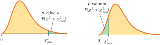
$\begin{array}{l} p -value = P (X^{2} > X_{data}^{2}) \\ Area to right of X_{data}^{2} \end{array}$

$\begin{array}{l} p -value = P (X^{2} < X_{data}^{2}) \\ Area to left of X_{data}^{2} \end{array}$

If $P (X^{2} > X_{data}^{2}) \leq 0.5$ , then

$χ_{data}^{2}$ is on the right side of the distribution
$p -value 2 \cdot P (χ^{2} > χ_{data}^{2})$

If $P (χ^{2} > χ_{data}^{2}) > 0.05$ , then

$χ_{data}^{2}$ is on the left side of the distribution
$p -value = 2 \cdot P (χ^{2} < χ_{data}^{2})$

Page 560

EXAMPLE 32 $χ^{2}$ test for $σ$ using the $p$ -value method and technology

The table contains the calories in ten entrée food items, courtesy of Food-A-Pedia. Test whether the population standard deviation is larger than 100 calories, using level of significance $α = 0.05$ .

entreecalories

Entrée item	Calories	Entrée item	Calories
Grilled steak	387	Ground beef (95% lean, medium patty)	167
Fried steak	440	Grilled pork chop (large)	314
Breaded fried steak	600	Fried pork chop (large)	326
Ground beef (75% lean, medium patty)	234	Meat pizza, thin crust, large	325
1 large BBQ short rib with sauce	148	Fried catfish (breaded or battered)	276

Solution

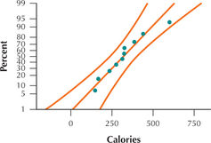
The normal probability plot in Figure 45 indicates acceptable normality, allowing us to proceed with the hypothesis test.

FIGURE 45 Normal probability plot of calories.

Step 1 State the hypotheses and the rejection rule.

The phrase “larger than” indicates that we have a right-tailed test. The question “Larger than what?” tells us that $σ_{0} = 100$ , giving us

$\begin{array}{l} H_{0} : σ = 100 & versus & H_{a} : σ > 100 \end{array}$

We reject $H_{0}$ if the $p-value \leq α = 0.05$ .
Step 2 Find $χ_{data}^{2}$ .

We use the Step-by-Step Technology Guide on page 562. The Minitab descriptive statistics in Figure 46 tell us that the sample variance is $s^{2} = 17, 742.5$ calories squared.

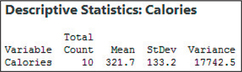FIGURE 46 Calories descriptive statistics.

Thus,

$χ_{data}^{2} = \frac{(n - 1) s^{2}}{σ_{0}^{2}} = \frac{(10 - 1) (17, 742.5)}{100^{2}} \approx 15.97$
Step 3 Find the $p$ -value.

For our right-tailed test, Table 14 tells us that

$p -value = P (χ^{2} > χ_{data}^{2}) = P (χ^{2} > 15.97)$

That is, the $p$ -value is the area to the right of $χ_{data}^{2} = 15.97$ , as shown in Figure 47. To find the $p$ -value, we use the instructions provided in the Step-by-Step Technology Guide provided at the end of this section. The TI-83/84 results shown in Figure 48 tell us that $p-value = P (χ^{2} > 15.97) = 0.0675107153 \approx 0.0675$ .

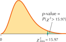FIGURE 47 $p$ -Value for $χ^{2}$ test

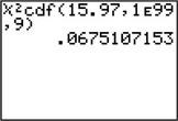FIGURE 48 TI-83/84 results.
Step 4 State the conclusion and the interpretation.

Because $p-value = 0.0675$ is not $\leq α = 0.05$ , we do not reject $H_{0}$ . There is insufficient evidence that the population standard deviation is greater than 100 calories.

NOW YOU CAN DO

Exercises 13–18.

Page 561

3 Using Confidence intervals for $σ$ to Perform Two-Tailed Hypothesis Tests for $σ$

Suppose we have a $100 (1 - α) %$ confidence interval for $σ$ , of the form (lower bound, upper bound), and are interested in two-tailed hypothesis tests using level of significance $α$ of the form:

$\begin{array}{l} H_{0} : σ = σ_{0} & versus & H_{a} : σ \neq σ_{0} \end{array}$

We will not reject $H_{0}$ for values of $σ_{0}$ that lie between the lower bound and upper bound of the confidence interval, and we will reject $H_{0}$ for values of $σ_{0}$ that lie outside this interval.

EXAMPLE 33 Using confidence intervals for $σ$ to conduct two-tailed $χ^{2}$ tests for $σ$

A 95% confidence interval for the population mean sodium content of breakfast cereals, in milligrams (mg) per serving, is given by

$(44.53 mg, 81.50 mg)$

Assume that the data are normally distributed. Test, using level of significance $α = 0.05$ , whether $σ$ differs from the following.

80 mg
40 mg

Solution

For the hypothesis test $H_{0} : σ = 80$ versus $H_{a} : σ \neq 80, σ_{0} = 80$ lies between the lower bound 44.53 and the upper bound 81.50 of the confidence interval, and we therefore do not reject $H_{0}$ . There is insufficient evidence that the population standard deviation of sodium content differs from 80 mg.
For the hypothesis test $H_{0} : σ = 40 versus H_{a} : σ \neq 40, σ_{0} = 40$ lies outside the confidence interval, and we therefore reject $H_{0}$ . There is evidence that the population standard deviation of sodium content differs from 40 mg.

NOW YOU CAN DO

Exercises 19–22.