3.4 Taxes
Governments at all levels (local, state, federal) tax all kinds of things, and they do it in different ways. Sometimes, suppliers are legally required to remit the tax. Stores in the United States collect sales taxes and send them to state revenue agencies, for example, just as producers in Canada and Europe collect and remit value-
In this section, we use the supply and demand model to show a striking finding of economics: In a competitive market, it doesn’t matter whether the buyer or the seller is required by law to actually sign the check and pay the tax to the government; the impact on consumers and producers is the same either way. We could change the law so that consumers paid sales tax instead of sellers, or employers paid the entire payroll tax, and market outcomes would not change. The total impact of a tax on consumers and sellers depends only on the steepness of the supply and demand curves, not on the identity of the payer. Before we can understand why this is true, however, we first need to look at how taxes affect a market.
Tax Effects on Markets
We start with a no-
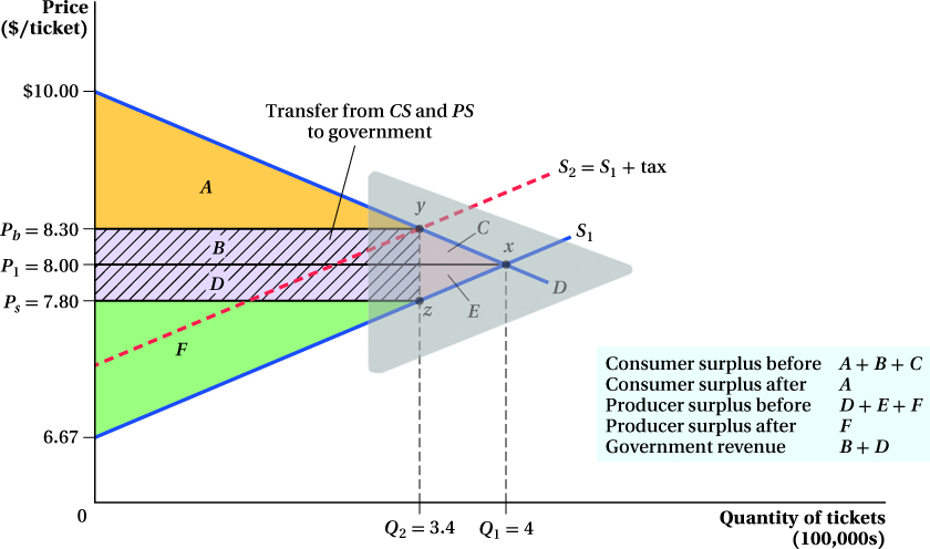
If it had been enacted, the tax would have required theater owners to pay 50 cents per ticket to the government. Let’s look at how such a change would affect the market for movie tickets. The tax is much like a 50-
But taxes do something different from a typical supply shift: They drive a wedge between the price buyers pay (the market price) and the price that producers actually receive (the market price minus the tax). With a normal supply curve, the price at any point on the supply curve is the price a producer receives for selling its product. With a tax, the product sells for the price Pb (we denote the price the buyers pay with a “b”), but the sellers only receive Ps (we denote the price the seller receives with an “s”). This is the buyers’ price minus the tax: Ps = Pb – tax. In other words, the buyers have to pay 50 cents more for any quantity, but the movie theaters don’t get to keep the extra money—
85
Because of this wedge, the new equilibrium in the Boston movie market involves two prices. The first, point y, is the price ($8.30) that the buyers pay at the theater that includes the 50-
There are two key characteristics to note about the post-
86
We can apply all the familiar concepts from consumer and producer surplus analysis to this new equilibrium. We just need to remember that the tax creates a second supply curve that we have to keep track of, rather than moving a single supply curve as before. The supply curve that the theater owner cares about is S1, the initial supply curve. The number of tickets that theaters are willing to supply at any particular price is still given by this curve, even after the tax is imposed, because the level of S1 reflects the after-
To make things clearer, let’s work through this example in more detail. In Figure 3.11, the demand curve for movie tickets in Boston is QD = 20 – 2P and the supply of movie tickets is QS = 3P – 20, where both quantities demanded and supplied in these curves are measured in hundreds of thousands of tickets. If the legislature passes the tax, all theater owners will be required to remit to the city 50 cents per ticket sold. We can analyze the tax’s effect on the market using graphs or equations.
Graphical Analysis With no taxes, solving the model our usual way gives a free-
The tax means buyers now face a new supply curve S2, equal to S1 shifted up by $0.50, the amount of the tax. This reduces the number of movie tickets bought in the market from 400,000 to 340,000. At that quantity, the price the buyers are paying rises from $8.00 to $8.30. Because the law requires suppliers (the theater owners) to pay the government a 50-
What happens to consumer and producer surplus in the post-
The new producer surplus is also smaller than before. Before the tax, it was D + E + F. After the tax, it is only F, the area above the supply curve and below the price that the suppliers receive after they pay the tax, $7.80.
Imposing the tax reduces total producer and consumer surplus from area (A + B + C ) + (D + E + F ) to just area A + F. Where has the surplus in areas B, C, D, and E gone? The area B + D is no longer consumer or producer surplus; it is government tax revenue, the tax times the quantity sold after the tax is implemented. With a tax, there is no surplus transfer between producers and consumers, as we saw in earlier examples. Instead, both producers and consumers transfer some of their surpluses to the government. This tax revenue is then “returned” to consumers and producers in the form of government services, so it is not lost.
Areas C and E are the deadweight loss from the tax. They are surpluses that moviegoers and theater owners formerly got from buying and selling tickets at the competitive price. This surplus is gone now because consumers buy fewer tickets at the higher post-
Just as in the price regulation cases, a natural way to look at the size of the deadweight loss is as a fraction of the surplus transfer. Before, that transfer occurred from producers to consumers (for a price ceiling) or from consumers to producers (for a price floor). Now, it’s from both to the government. The ratio in this case is the area C + E to the area B + D, which is the DWL as a share of revenue.
87
Analysis Using Equations The no-
QD = QS
20 – 2P = 3P – 20
5P = 40
P1 = 40/5 = $8 per ticket
QD = 20 – 2($8) = 4 or QS = 3($8) – 20 = 4
Therefore, before the tax, the equilibrium price is $8 and 400,000 tickets are sold.
The pre-

Again, the choke price is found by determining the price that pushes the quantity demanded to zero:
QD = 20 – 2PDChoke = 0
PDChoke = $10
In other words, this demand curve says that if tickets cost $10, no one will go to theaters in the city of Boston (perhaps because theaters in the suburbs are an attractive alternative).
Plugging the demand choke price into the CS formula gives a consumer surplus of

The producer surplus is the triangle above the supply curve and below the price:

The supply choke price is the price that moves quantity supplied to zero:
QS = 3PSChoke – 20 = 0
PSChoke = $6.67
That is, at any price below $6.67 a ticket, no theaters would operate in Boston. Plugging this supply choke price into the PS formula gives a producer surplus of

What happens to consumer and producer surplus if Mayor Menino applies his 50-
88
To solve for the post-
QD = QS
20 – 2Pb = 3Ps – 20
20 – 2(Ps + 0.50) = 3Ps – 20
20 – 2Ps – 1 = 3Ps – 20
5Ps = 39
Ps = 39/5 = $7.80
Therefore, the buyers face the following price:
Pb = Ps + 0.50 = $7.80 + 0.50 = $8.30
Now if we plug the buyer price into the demand curve equation and the supplier price into the supply curve equation, they will both give the same after-
Q2 = 20 – 2(8.30) = 3.4
or
Q2 = 3(7.80) – 20 = 3.4
Only 340,000 tickets will be sold once the tax is put into place.
The consumer surplus after a tax is the area below the demand curve but above the price that the buyers pay:

The producer surplus is the area above the supply curve and below the price that the suppliers receive:

So the tax makes consumer surplus fall by $111,000 and producer surplus fall by $74,000 from their values in the no-
Revenue = $0.50Q2
= $0.50(340,000) = $170,000
Notice that the total amount of the lost surplus, $185,000, is more than the amount of revenue that the government generated, $170,000. The difference of $15,000 is the deadweight loss of the tax.
A different way to calculate DWL is to compute the area of the triangle whose base is the change in quantity and whose height is the amount of the tax:

FREAKONOMICS
Unintended Consequences of a Tax on Garbage
89
South Norfolk is an idyllic area nestled in the eastern part of England. If you happened to be visiting there in 2005, you would have seen charming villages, cattle grazing in the fields, the occasional castle on a hill, and piles of garbage (or as they say in South Norfolk, “rubbish”) strewn haphazardly along the side of the road.
It’s not that the citizens of South Norfolk are generally filthy slobs; if you had visited the area the year before, there would have been cows and castles, but almost no trash on the side of the road.
What happened? The government used simple economic tools to fight a problem. And they worked. Too well.
Collecting trash is a government responsibility, and there is a cost associated with collecting trash and putting it in landfills. Governments usually pay for this cost by charging citizens lump sum fees; one payment buys any amount of trash removal someone needs, large or small. As a result of this practice of not taxing trash on the margin, people don’t pay the full cost of the garbage they produce, and they produce too much garbage as a result. The obvious economic solution is to charge people by the amount of trash they produce. And this is exactly what the South Norfolk District Council aimed to do when it initiated a trial run of this policy in 2005. The local government placed microchips in garbage bins, with plans to tax citizens by the weight of trash in the bins as measured by the microchips.

So why did a lot of trash end up by the side of the road? South Norfolk citizens realized that they could get around the potential tax by fly-
Tax evasion doesn’t always work out as planned, however. Ireland also recently introduced a pay-
*S. M. Murphy, C. Davidson, A. M. Kennedy, P. A. Eadie, and C. Lawlor, “Backyard Burning,” Journal of Plastic, Reconstructive & Aesthetic Surgery 61, no. 2 (2008): 180–
The broader lesson here is an important one: When you provide strong incentives, people react strongly. They change their behavior not only in the way you want them to, but in all sorts of other ways that you might prefer they hadn’t. One of the characteristics that distinguishes a great economist from a not-
90
That’s about 9% of the revenue generated by the tax. In other words, this tax burns up about $1 of surplus in DWL for every $11 of revenue it generates.
Why Taxes Create a Deadweight Loss
Just as we showed in the case of price and quantity regulations, the main determinant of the DWL from a tax as a share of revenue is how much the quantity changes when the tax is added. The size of that change depends, in turn, on how sensitive supply and demand are to prices. The deadweight loss from pizza price controls, for example, came about because there were consumers and suppliers who would like to trade at market prices and would have earned surplus from doing so, but were prevented from engaging in these transactions by the price ceiling. With taxes, there are no forbidden transactions. The source of the loss is the same, however. There are people who would have bought tickets at the market price without a tax and would have gained some surplus from doing so. Once the government adds a tax, the after-
Why a Big Tax Is Much Worse Than a Small Tax
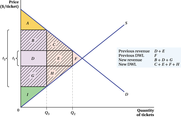
An interesting result of our analysis is that it implies the inefficiency represented by the size of the deadweight loss gets much bigger as the size of a tax becomes larger. In the movie ticket tax example (Figure 3.11), we saw that the DWL from the tax was area C + E and that the revenue generated was B + D. What would happen if Mayor Menino decided to increase the ticket tax? How much more revenue and how much more DWL would this tax increase create?
Figure 3.12 illustrates the outcome for a general case. The larger tax reduces the quantity even further, from Q2 to Q3. The DWL under the larger tax is area C + E + F + H (remember that it was only area F with the smaller tax). Government revenue, which was area D + E with a smaller tax, is now area B + D + G. That is, the government gains areas B and G because the people who still buy tickets are paying more in taxes. However, the government loses area E, because some people stop buying movie tickets after the tax is raised. If we look at the DWL as a share of the revenue generated, it is clear that the incremental revenue generated by increasing this tax causes more inefficiency than the smaller tax did. Initially, the DWL was F, with a revenue gain of D + E. But the incremental DWL here is C + E + H, while the revenue gain is only B + G – E. In fact, if taxes become high enough, the increase in revenue per ticket from the tax will be more than offset by the reduction in the quantity of tickets sold, and there will be no revenue gain at all!
A general rule of thumb is that the DWL of a tax rises with the square of the tax rate.10 That is, doubling the tax rate quadruples the DWL. That’s why economists tend to favor tax policies that exhibit what is called “low rates and broad bases.” That is just a way of saying that, all else equal, taxing ten things at a low rate is better than taxing five things at zero and five things at a high rate. Because DWL rises with the square of the tax rate, the overall DWL will be larger with the five high rates than with the ten low rates.
91
The Incidence of Taxation: The Payer Doesn’t Matter
tax incidence
Who actually pays a tax.
An important thing to note about the movie ticket example is that although we supposed that it would be the theater owners who were legally obligated to remit the 50 cents per ticket tax to the City of Boston, they don’t bear the complete burden of the tax. Before the tax came in, the theater owners received $8 per ticket and moviegoers paid $8 a ticket. After the $0.50 tax, moviegoers pay $8.30 a ticket. After they send in the tax, however, the theaters only end up with $7.80 per ticket. Therefore, of the 50 cents going to the government, 30 cents (60%) of it is coming out of consumers’ pockets because their price went up by 30 cents. Movie theaters send the tax check to the government, but they are able to pass on much of the tax to consumers through higher prices. This means that the price realized by the suppliers goes down by only 20 cents. Who really bears the burden of a tax is called tax incidence. The incidence of this tax is 60% on the buyers and 40% on the suppliers.
92
Now let’s say Boston changed the rule for who pays the tax to the government. Instead of the theater sending the tax payment to the government, moviegoers would pay the tax by, after buying their ticket at whatever price the theater charges, dropping two quarters in a “Menino Box” as they enter the theater (silly idea, yes, but this is just to make a point).
This does not alter the tax incidence. The equations below show that in the tax formula it doesn’t matter whether you subtract the tax from what the supplier receives or add the tax to what the buyer pays. Ps = Pb – tax is the same as Ps + tax = Pb.
This can also be seen graphically. The original case where the theater remits the tax is shown in Figure 3.13a. When the tax is instead paid by buyers, their quantity demanded depends on the price including the tax. But the price suppliers receive at this quantity demanded is only the price without the tax. To account for this difference, we shift down the demand curve by the amount of the tax, from D1 to D2 in Figure 3.13b. But the result hasn’t changed: Quantity demanded is still Q2, and the difference between the buyer’s price and the seller’s price still equals the amount of the tax. Thus, the incidence of a tax does not depend on who is legally bound to pay it.
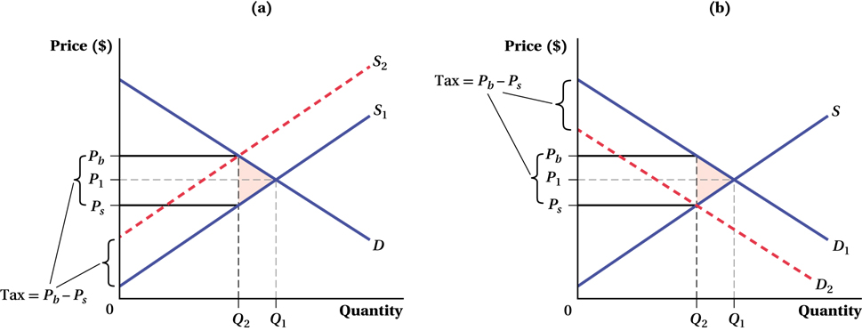
(b) When the buyer pays the tax, the demand curve shifts inward by the amount of the tax, Pb – Ps, from D1 to D2. The equilibrium quantity decreases from Q1 to Q2. As in panel a, the seller now faces price Ps at the equilibrium, while the buyer pays price Pb.
That’s why a helpful way to picture taxes on a graph is to just forget about whether the tax is moving the supply curve up or the demand curve down. Instead, start from the initial no-
This point about tax incidence is fundamental. If you have ever had a job, you probably know that the government takes many taxes out of your pay. Some of these are payroll taxes that appear on your pay stub as FICA (Federal Insurance Contributions Act). They are collected to pay for Social Security and Medicare. In the United States, payroll taxes are legally split evenly between workers and employers. In other words, if you earn wages of $1,000, you have to pay 7.65% of that in payroll taxes and the employer has to pay another 7.65% on its own.11 Would U.S. workers be better or worse off if the law changed so that the company paid 15.3% and workers paid nothing, or if it instead made the employee pay 15.3% and his or her employers paid nothing? The analyses we’ve just completed suggest that such changes wouldn’t make any difference. In a competitive market, the wage would adjust to the same level regardless of which side of the market is legally bound to pay the tax.
93
It turns out that the only thing that matters about the economic effects of this tax is how elastic the supply and the demand for labor are. To see why, let’s consider the two extremes.
make the grade
Did I measure deadweight loss correctly?
A few simple tricks will help you nail problems involving deadweight loss. First, whenever the quantity consumed falls as a result of a government policy, a deadweight loss occurs. (This isn’t exactly correct; if externalities are present, government policies can actually improve market outcomes. We learn more about externalities in Chapter 17.) If the quantity doesn’t become distorted, no deadweight loss occurs. Second, the deadweight loss almost always takes the shape of a triangle, and moreover, that triangle points at the efficient market equilibrium with no market distortion. Why? Because deadweight loss measures the consumer and producer surplus destroyed. As we have seen, this loss in surplus grows as we move further and further away from the efficient equilibrium. The growing distance between the sides of the triangle reflects this fact.
Relatively Elastic Demand with Relatively Inelastic Supply In a market characterized by relatively elastic demand and inelastic supply, buyers are very sensitive to price and the suppliers are not. Most labor economists tend to think of the labor market in this way, so that the 15.3% FICA tax (the combined tax rate on the two sides) applies to a market in which labor supply is fairly inelastic (people work a similar amount even if their wage goes up or down) and firms’ demand for labor is fairly elastic. This market is illustrated in Figure 3.14a.
Applying the methods we’ve used throughout this section, we see that the tax is borne almost entirely by the suppliers—
94
Relatively Inelastic Demand with Relatively Elastic Supply Figure 3.14b shows a market characterized by relatively inelastic demand (buyers are not sensitive to price) and elastic supply (suppliers are very sensitive to price). In the market for cigarettes, for instance, many buyers are addicted and tend to buy a similar amount no matter how much the price goes up. Cigarette supply is more elastic. You can see in the figure that in this case, consumers bear the brunt of the tax. A tax on cigarettes causes the buyers’ price to rise from P1 to Pb, almost the entire amount of the tax. Suppliers are only a bit worse off than they were before, because they can pass on the higher costs to the inelastic consumers.
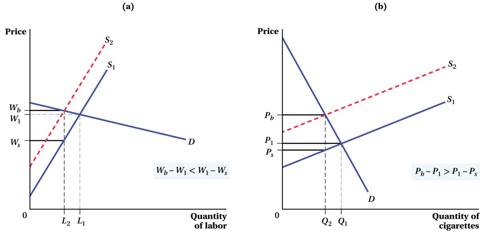
(b) In the market for cigarettes where demand is inelastic and supply elastic, we begin with supply curve S1, demand D, and equilibrium price and quantity (P1, Q1). The implementation of the tax, Pb – Ps, shifts the supply curve inward from S1 to S2 and decreases the equilibrium quantity of cigarettes from Q1 to Q2. Because smokers in this market are not very sensitive to price and cigarette companies are, the effect of the tax on the price consumers pay is much larger than its effect on the price companies receive, Pb – P1 > P1 – Ps.
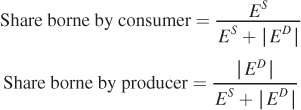
We could do this entire analysis using equations, as we did in the movie ticket example. It turns out that there is a general formula that will approximate the share of the tax borne by the consumer and the share borne by the producer. Not surprisingly given what we’ve just discussed, these shares depend on elasticities:
95
If the price elasticity of supply (ES) is infinite, the consumers’ share is equal to 1; that is, consumers bear the whole burden when supply is perfectly elastic. If the absolute value of the price elasticity of demand  is infinite, the consumers’ share of the tax burden is zero, and suppliers bear the whole burden of the tax.
figure it out 3.3
Consider the demand and supply for cola in a market represented by the following equations:
QD = 15 – 10P
QS = 40P – 50
where Q is millions of bottles per year and P measures dollars per bottle. The equilibrium price of cola is $1.30 per bottle, and 2 million bottles are sold each year.
Calculate the price elasticity of demand and the price elasticity of supply at the equilibrium price and quantity.
Calculate the share of a tax that would be borne by consumers and the share borne by producers.
If a tax of $0.15 per bottle is created, what would be the expected price buyers will have to pay? What price will sellers receive after the tax?
Solution:
The formula for price elasticity of demand is

From the demand curve, we can calculate
 . Each time P changes by 1 unit, QD falls by 10. Therefore,
Substituting into the formula for elasticity, we get

The formula for price elasticity of supply is

From the supply curve, we can see that
 .
.Note that each time P increases by 1 unit, QS rises by 40.
Thus, the price elasticity of supply is

The proportion of the tax borne by buyers will be

The proportion of the tax borne by sellers will be

So buyers will bear 80% of the tax and sellers will bear only 20% of the tax.
If there is a tax of $0.15 per bottle, buyers will bear 80% of the tax:
Increase in Pb = (0.80)($0.15) = $0.12
The price buyers pay will rise from $1.30 per bottle (the original equilibrium price) to $1.42.
Sellers will bear the other 20% of the tax:
Decrease in Ps = (0.2)($0.15) = $0.03
The price sellers receive will fall from $1.30 per bottle to $1.27.
 See the problem worked out using calculus