7.4 Average and Marginal Costs
Understanding the total cost curve (and its fixed and variable cost components) is an important part of analyzing firms’ production behavior. To see why, we introduce two other cost concepts that play a key role in production decisions: average cost and marginal cost. In our Chapter 6 analysis of a firm’s production decisions, we took the firm’s desired output level as given. In the next few chapters, we will see that average and marginal costs are important in determining a firm’s desired output level.
259
Average Cost Measures
average fixed cost (AFC)
A firm’s fixed cost per unit of output.
Average cost is fairly straightforward. It’s just cost divided by quantity. Because there are three costs (total, fixed, and variable), there are three kinds of average cost. Each of these measures examines the per-
260
AFC = FC/Q
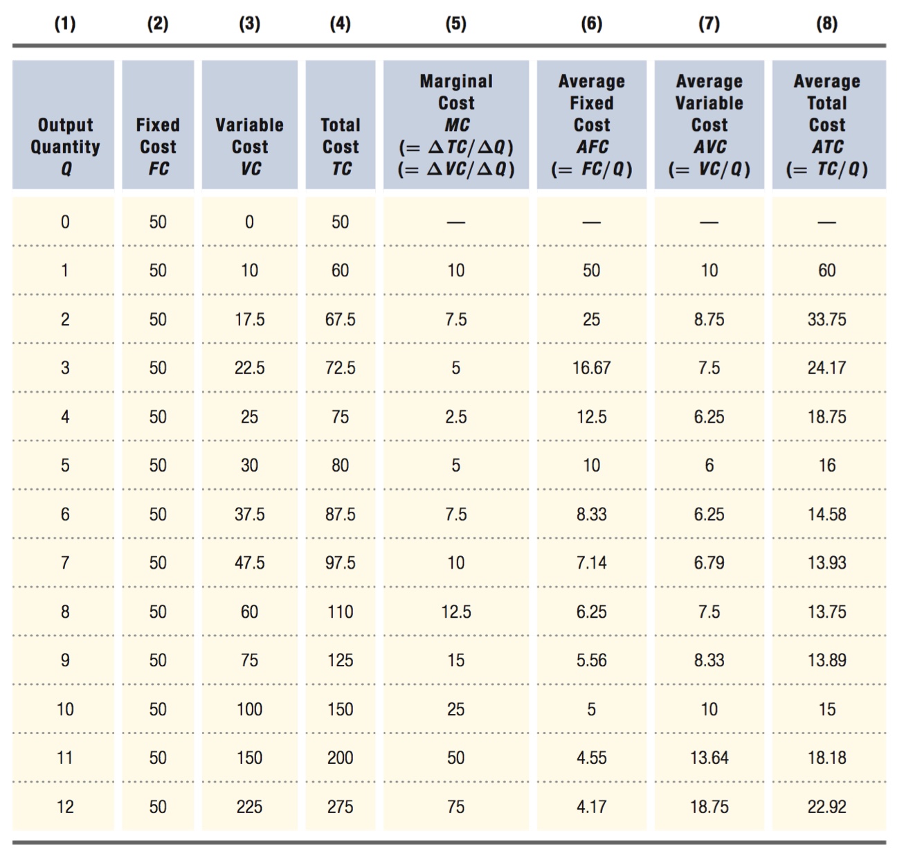
Column (6) of Table 7.2 shows average fixed cost AFC for Fleet Foot (FF). AFC falls as output rises. The numerator (fixed cost) is constant while the denominator (quantity) rises, so average fixed cost becomes smaller and smaller as quantity goes up. (The fixed cost is spread over more and more units of output.) Thus, as FF manufactures more running shoes, the average fixed cost it pays per pair of shoes declines.
average variable cost
A firm’s variable cost per unit of output.
Average variable cost measures the per-
AVC = VC/Q
Unlike average fixed cost, average variable cost can go up or down as quantity changes. In this case, it declines until five units are produced, after which it rises, leading to a U-
average total cost
A firm’s total cost per unit of output.
Average total cost is total cost TC per unit of output Q:
ATC = TC/Q
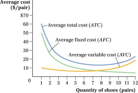
Average total cost for Fleet Foot is shown in the last column of Table 7.2. For FF, average total cost at first falls and then rises as output rises. Firms’ average total costs often exhibit this sort of U-
ATC = TC/Q = (FC + VC)/Q
= FC/Q + VC/Q
= AFC + AVC
Average total cost first falls as output rises because the dominant influence on average total cost is the rapidly declining average fixed cost. But as output continues to rise, average variable cost keeps increasing, first slowing the rate at which average total cost is falling and eventually causing average total cost to increase with output. These changes create a U-
261
FREAKONOMICS
3D Printers and Manufacturing Cost
Star Trek is full of far-
As crazy as it sounds, though, the “replicator” is no longer science fiction. We don’t call such products replicators, but rather 3D printers. 3D printers take raw materials such as plastic and gold and convert them into forks and knives for your dining room table or an eccentric sculpture for your living room. The new “Foodini” 3D printer can even print food, a Trekkie’s dream come true. If their cost falls enough, 3D printers will become as common as microwave ovens or toasters. Instead of going to the store to buy food or ordering a meal online, you will simply punch a few buttons and manufacture the desired items right in your own home.
As with many new technologies, the costs right now are extremely high. The fixed costs of a commercial-
As unlikely as it seemed in 1910 that the assembly line would replace master craftsmen, it happened. The same was the case with laptops and cell phones, which were science fiction 50 years ago. What was once conceivable only in the world of Star Trek might soon be a regular part of your daily life. You may have to wait just a bit longer, though, to acquire a transporter beam for your living room.
Marginal Cost
marginal cost
The cost of producing an additional unit of output.
The other key cost concept is marginal cost, a measure of how much it costs a firm to produce one more unit of output:
MC = ΔTC/ΔQ
where ΔTC is the change in total cost and ΔQ is a 1-
Fleet Foot’s marginal cost is shown in the fifth column of Table 7.2. It is the difference in total cost when output increases by 1 pair of shoes. But notice something else: Marginal cost also equals the difference in variable cost when one additional unit is produced. That’s because, by definition, fixed cost does not change when output changes. Therefore, fixed cost does not affect marginal cost; only variable cost changes when the firm produces one more unit. This means marginal cost can also be defined as the change in variable cost from producing another unit of output:
MC = ΔVC/ΔQ (= ΔTC/ΔQ)
For this reason, marginal cost is not split into fixed and variable cost components, as is average cost. Marginal cost is only marginal variable cost.
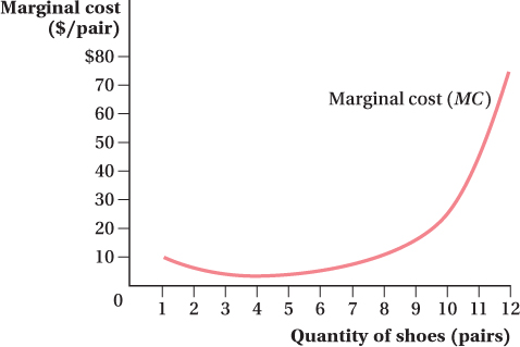
Fleet Foot’s marginal cost initially declines as output increases. After a certain output level (4 units in Table 7.2), marginal cost begins to rise, and at even higher output levels, it rises steeply. Why? Marginal cost may initially fall at low quantities because complications may arise in producing the first few units that can be remedied fairly quickly, or because having more scale allows workers to specialize in those tasks that they are best at. As output continues to increase, however, these marginal cost reductions stop and marginal cost begins to increase with the quantity produced, as seen in Figure 7.3. There are many reasons why it becomes more and more expensive to make another unit as output rises: Capacity constraints may occur, inputs may become more expensive as the firm uses more of them, it may be harder for the company to coordinate its operations, and so on.
262
Understanding the concept of marginal cost is critical: It is one of the most central concepts in all of economics, and it is the only cost that matters for many of the key decisions a firm makes.
 See the problem worked out using calculus
figure it out 7.2
Fields Forever is a small farm that grows strawberries to sell at the local farmers’ market. It produces strawberries using 5 acres of land that it rents for $200 per week. Fields Forever also hires labor at a price of $250 per week per worker. The table below shows how the output of strawberries (measured in truckloads) varies with the number of workers hired:
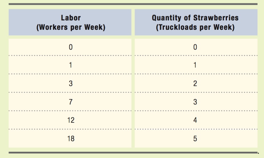
Calculate the marginal cost of 1 to 5 truckloads of strawberries for Fields Forever.
Solution:
263
The easiest way to solve this problem is to add several columns to the table on the previous page. We should add fixed cost, variable cost, and total cost. Fixed cost is the cost of land that does not vary as output varies. Therefore, fixed cost is $200. Variable cost is the cost of labor. It can be found by multiplying the quantity of labor by the wage rate ($250). Total cost is the sum of fixed cost and variable cost.
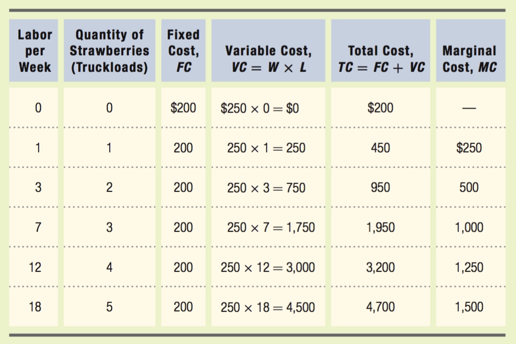
Marginal cost is the change in total cost per unit increase in output, or ΔTC/ΔQ. When output rises from 0 units to 1 truckload of strawberries, total cost rises from $200 to $450. Therefore, the marginal cost of the first truckload of strawberries is $450 – $200 = $250. As output rises from 1 to 2 truckloads, total cost rises from $450 to $950, so the marginal cost is $950 – $450 = $500. When the third truckload is produced, total cost rises from $950 to $1,950, so marginal cost is $1,950 – $950 = $1,000. Production of the fourth truckload pushes total cost to $3,200, so the marginal cost of the fourth truckload is $3,200 – $1,950 = $1,250. When production rises from 4 to 5 truckloads, total cost rises from $3,200 to $4,700, so the marginal cost of the fifth truckload is $1,500.
We could have also calculated the marginal cost of each truckload by looking at only the change in variable cost (rather than the change in total cost). Because the amount of land is fixed, Fields Forever can only grow more strawberries by hiring more labor and increasing its variable cost.
Relationships between Average and Marginal Costs
Because average cost and marginal cost are both derived from total cost, they are directly related. If the marginal cost of output is less than the average cost at a particular quantity, producing an additional unit will reduce the average cost because the extra unit’s cost is less than the average cost of making all the units before it. (This relationship is the same as that between the average and marginal products of labor we learned about in Chapter 6.) Suppose, for example, that a firm had produced 9 units of output at an average cost of $100 per unit. If the marginal cost of the next unit is $90, the average cost will fall to ($900 + $90)/10 = $99, because the marginal cost of that extra unit is less than the average cost of the previous units.
264
This means that if the marginal cost curve is below an average cost curve at some quantity, average cost must be falling—
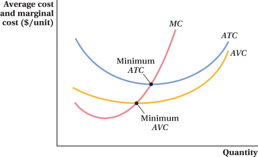
You can see this relationship in Figure 7.4, which shows an average total cost curve, an average variable cost curve, and a marginal cost curve all derived from a single total cost curve. At lower quantities, when the marginal cost curve is below the average cost curves, the average cost curves are downward-
When the marginal cost of the additional unit is above average cost, then producing it increases the average cost. Therefore, if the marginal cost curve is above an average cost curve at a quantity level, average cost is rising, and the average cost curve slopes up at that quantity. Again, this is true for both average total cost and average variable cost. This property explains why average variable cost curves and average total cost curves often have a U-
The only point at which there is no change in average cost from producing one more unit occurs at the minimum point of the average variable and average total cost curves, where marginal and average cost are equal. These minimum points are indicated on Figure 7.4. (In the next chapter, we see that the point at which average and marginal costs are equal and average total cost is minimized has a special significance in competitive markets.)
265
figure it out 7.3
Suppose a firm’s total cost curve is TC = 15Q2 + 8Q + 45, and MC = 30Q + 8.
Find the firm’s fixed cost, variable cost, average total cost, and average variable cost.
Find the output level that minimizes average total cost.
Find the output level at which average variable cost is minimized.
Solution:
Fixed cost is a cost that does not vary as output changes. We can find FC by calculating total cost at 0 units of output:
TC = 15(0)2 + 8(0) + 45 = 45
Variable cost can be found by subtracting fixed cost from total cost:
VC = TC – FC = (15Q2 + 8Q + 45) – 45 = 15Q2 + 8Q
Notice that, as we have learned in the chapter, VC depends on output; as Q rises, VC rises.
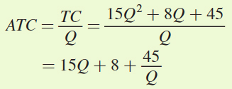
Average total cost is total cost per unit or TC/Q:
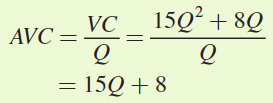
Average variable cost is variable cost per unit or VC/Q:
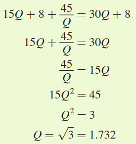
Minimum average total cost occurs when ATC = MC:
Minimum average variable cost occurs where AVC = MC:
15Q + 8 = 30Q + 8
15Q = 0
Q = 0