7.5 Short-Run and Long-Run Cost Curves
Earlier in this chapter, we discussed how time horizons affect fixed and variable costs. Over longer periods of time, a firm has more ability to shift input levels in response to changes in desired output, making even “heavy-duty” capital inputs such as factories more flexible. In turn, this flexibility renders the firms’ costs more variable and less fixed.
Recall from Chapter 6 that we defined the short-run production function as having a fixed level of capital, ; that is,
 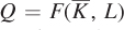 . In the long-run production function, Q = F(K, L), capital can adjust. There is a related distinction in cost curves. Short-run cost curves relate a firm’s production cost to its quantity of output when its level of capital is fixed. Long-run cost curves assume that a firm’s capital inputs can change just as its labor inputs may.
Short-Run Production and Total Cost Curves
short-run total cost curve
The mathematical representation of a firm’s total cost of producing different quantities of output at a fixed level of capital.
A firm’s short-run total cost curve shows the firm’s total cost of producing different quantities of output when it is stuck at a particular level of capital
. Just as there is a different short-run production function for every possible level of capital, so too is there a different short-run total cost curve for each capital level.
In Chapter 6, we saw that a firm’s total cost curve (which relates cost and quantity of output) is related to its expansion path (which relates cost-minimizing input combinations to output). This relationship holds true in both the long run and the short run. However, in the short run, we must remember that a firm has only a fixed level of capital. Therefore, to examine how the firm minimizes its cost in the short run, we must examine the firm’s expansion path given its fixed capital. Let’s return to Ivor’s Engines, the firm we looked at in Section 6.7. Figure 7.5 shows the same isoquants and isocost lines we used to construct the long-run expansion path in Chapter 6. In the short run, Ivor’s has a fixed capital level, and the expansion path is a horizontal line at that capital level. In the figure, we’ve assumed  . If the firm wants to adjust how much output it produces in the short run, it has to move along this line. It does so by changing its labor inputs, the only input it can change in the short run.
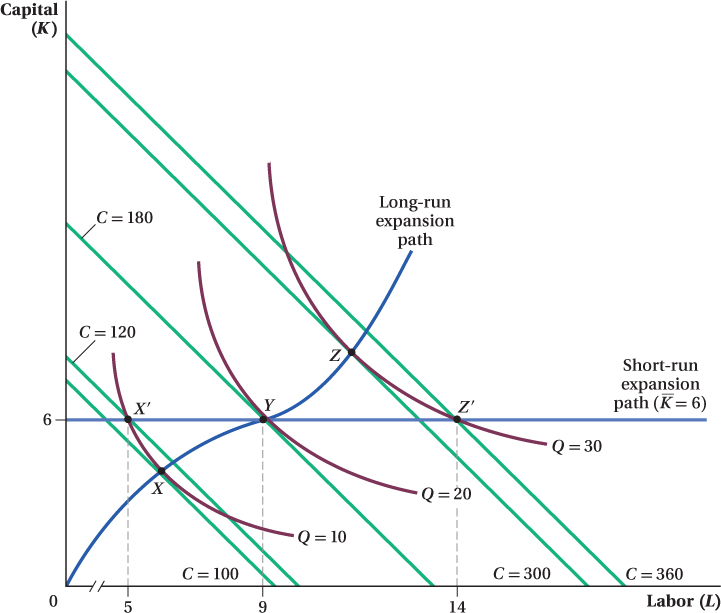
Figure 7.5: Figure 7.5 Long-Run and Short-Run Expansion Path for Ivor’s Engines
Figure 7.5: Along Ivor’s Engines long-run expansion path, the firm can change its level of capital. Along Ivor’s short-run expansion path, capital is fixed at 6, and the expansion path is horizontal at
. Ivor’s Engines can change its output quantity only by changing the quantity of labor used. At points X′, Y, and Z′, Ivor’s Engines minimizes cost in the short run by using 5, 9, and 14 laborers to produce 10, 20, and 30 engines at a cost of $120, $180, and $360, respectively. At Q = 20, the cost-minimizing capital and labor combination, Y, is the same in the long run and short run, and production cost is the same ($180). At Q = 10 and Q = 30, production is more expensive in the short run than in the long run.
Suppose Ivor’s Engines initially produces 20 units, as shown by the isoquant Q = 20. Suppose also that the cost of producing 20 engines is minimized when 6 units of capital are employed. That is, the Q = 20 isoquant is tangent to the C = $180 isocost line at point Y, when Ivor’s capital inputs are 6. (We can justify this assumption by imagining that in the past, when it had the ability to change its capital input levels, Ivor’s was making 20 engines and chose its optimal capital level accordingly.) The labor input level that minimizes the cost of producing 20 engines is L = 9 units.
To see the difference between short-run and long-run cost curves, compare the points on the isoquants on the short-run (fixed-capital) expansion path to those on the long-run (flexible-capital) expansion path. For an output level of 20 engines, these are the same (point Y) because we have assumed that a capital level of
was cost-minimizing for this quantity.
For the Q = 30 isoquant, however, the short-run and long-run input combinations are different. In the short run when capital is fixed at 6 units, if the firm wants to produce 30 units, it has to use the input combination at point Z′, with 14 units of labor. But notice that Z′ is outside (i.e., further from the origin than) the C = $300 isocost line that is tangent to the long-run cost-minimizing input combination at point Z (which uses 11 units of labor). Instead, Z′ is on the C = $360 isocost line. In other words, it is more expensive for Ivor’s Engines to produce 30 engines in the short run, when it cannot adjust its capital inputs. This is because it is forced to use more labor and less capital than it would if it could change all of its inputs freely.
The same property holds true if Ivor’s wants to make 10 engines. With capital fixed in the short run, the firm must use the input combination at point X′ (with 5 units of labor). This point is on the C = $120 isocost line, while the flexible-capital cost-minimizing input combination X is on the C = $100 isocost line. So again, the firm’s short-run total costs are higher than its long-run total costs. Here, it is because Ivor’s is forced to use more capital than it would if it could adjust its capital inputs.
While we only looked at two quantities other than 20 engines, this general pattern holds at all other quantities. Whether Ivor’s Engines wants to make more or fewer than 20 engines (the output level at which short- and long-run costs are the same), its total costs are higher in the short run than in the long run. Restricting the firm’s ability to freely choose its capital input necessarily increases its costs, except when Q = 20 and the current level of capital and labor happens to be optimal.
If we plot the total cost curves that correspond to these short- and long-run expansion paths, we arrive at Figure 7.6. The long-run total cost curve TCLR is the same as when we assumed the firm was free to adjust all inputs to minimize costs. At Q = 20 engines, this curve and the short-run total cost curve TCSR overlap because we assumed that capital was at the cost-minimizing capital level at this quantity. (We’ve labeled this point Y because it corresponds to the quantity and total cost combination at point Y in Figure 7.5.) For every other quantity, however, the short-run (fixed-capital) total cost curve is higher than the long-run (flexible-capital) total cost curve. Note that short-run total costs are positive when Q = 0 but zero in the long run. In other words, there are fixed costs in the short run but not in the long run when all inputs are flexible.
Figure 7.6: Figure 7.6 Short-Run and Long-Run Total Cost Curves for Ivor’s Engines
Figure 7.6: The short-run total cost curve (TCSR) for Ivor’s Engines is constructed using the isocost lines from the expansion path in Figure 7.5. At Y, when Q = 20, TCSR and the long-run total cost curve (TCLR) overlap. At all other values of Q, including Q = 10 and Q = 30, TCSR is above TCLR, and short-run total cost is higher than long-run total cost. This is also true when Q = 0 since some input costs are fixed in the short run, while in the long run, all inputs are flexible.
Short-Run versus Long-Run Average Total Cost Curves
From the total cost curves in Figure 7.6, we can construct Ivor’s Engines long-run and short-run average total cost curves. These are shown in Figure 7.7. The long-run average total cost curve is ATCLRand the short-run average total cost curve ATCSR,20. (We add the “20” subscript to denote that the curve shows the firm’s average total cost when its capital is fixed at a level that minimizes the costs of producing 20 units of output.)
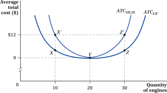
Figure 7.7: Figure 7.7 Short-Run and Long-Run Average Total Cost Curves for Ivor’s Engines
Figure 7.7: The short-run average total cost curve (ATCSR,20) and the long-run average total cost curve (ATCLR) are constructed using TCSR and TCLR from Figure 7.6. At Y, when Q = 20 and the cost-minimizing amount of capital is 6 units, the ATCSR and ATCLR both equal $9. At all other values of Q, including Q = 10 and Q = 30, ATCSR is above ATCLR, and short-run average total cost is higher than long-run average total cost.
As with the total cost curves, the short- and long-run average total cost curves overlap at Q = 20 engines, because that’s where the firm’s fixed capital level of 6 units is also cost-minimizing. Here, long-run and short-run average total costs are $180/20 = $9.
For all other output quantities, short-run average total cost is higher than long-run average total cost. Short-run total cost is higher than long-run total cost at every other quantity. Because average total cost divides these different total costs by the same quantity, average total cost must be higher in the short run, too. When Ivor’s is making 30 engines with capital fixed at 6 units, its total costs are $360, and its short-run average total cost is $12 per unit. When it makes 10 engines, short-run average total cost is $120/10 = $12 per unit as well. These points on the short-run average total cost curve ATCSR,20 are labeled Z′ and X′ to correspond to the analogous points on the short-run total cost curve in Figure 7.6. The long-run average total costs at 10 and 30 units are labeled Z and X, and these correspond to the similarly labeled points in Figure 7.6.
Up to this point, we’ve analyzed the distinction between long-run and short-run total and average total costs assuming that the short-run level of capital was fixed at 6 units, the level that minimized the cost of producing 20 engines. But suppose capital had been fixed at some other level instead. To be concrete, let’s say it was fixed at 9 units of capital, the level that minimizes the cost of producing 30 engines. (This is the capital level at point Z in Figure 7.6.)
The analysis is exactly the same as above. The long-run total and average total cost curves don’t change, because the firm will still choose the same capital inputs (resulting in the same costs) given its flexibility in the long run. However, the short-run cost curves change because the fixed level of capital has changed. By the same logic as above, the short-run total and average total cost curves will be above the corresponding long-run curves at every quantity except one. In this case, though, rather than overlapping at 20 units of output, it overlaps at Q = 30, because capital is now fixed at the cost-minimizing level for 30 engines. The logic behind why short-run total and average total costs are higher at every other quantity than 30 is the same: Not allowing the firm to change its capital with output raises the cost of producing any quantity except when the firm would have chosen that capital level anyway.
We can make the same comparisons with capital held fixed at 4 units, which minimizes the costs of producing 10 engines (corresponding to point X in Figure 7.6). Again, the same patterns hold. The short-run total and average total cost curves are higher at every quantity except Q = 10.
These other short-run average total cost curves are shown in Figure 7.8 along with ATCSR,20 and the long-run average total cost curve ATCLR from Figure 7.7. ATCSR,10 and ATCSR,30 show short-run average costs when the firm has a fixed capital level that minimizes the total costs of making 10 and 30 engines, respectively. As you can see in Figure 7.8, the long-run average total cost curve connects the locations (only one per fixed capital level) at which the short-run average total cost curves touch the long-run curve. We could repeat our short-run analysis with capital held fixed at any level, and the short-run average total cost curve will always be higher than the long-run curve, except in one point. If we drew out every such short-run average total cost curve, they would trace the long-run average total cost curve just like the three we have shown in the figure. As economists say, the long-run average total cost curve is an “envelope” of short-run average total cost curves, because the long-run average total cost curve forms a boundary that envelops all possible short-run average total cost curves, as seen in Figure 7.8.
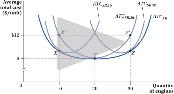
Figure 7.8: Figure 7.8 Long-Run Average Total Cost Curve Envelops the Short-Run Average Total Cost Curves
Figure 7.8: ATCSR,10 and ATCSR,30 show short-run average costs when the firm has a fixed capital level that minimizes the total costs of making 10 and 30 engines, respectively. With  and
and  , ATCSR,10 and ATCSR,30 overlap ATCLR at the cost-minimizing points X and Z, respectively. However, X and Z are not at the lowest points on ATCSR,10 and ATCSR,30 because the output levels that minimize ATCSR,10 and ATCSR,30 can be produced more cheaply if capital inputs are flexible.
One interesting thing to notice about Figure 7.8 is that ATCSR,10 and ATCSR,30 do not touch ATCLR at their lowest points. That’s because even the output levels that minimize average total costs in the short run when capital is fixed (the low points on ATCSR,10 and ATCSR,30) can be produced more cheaply if capital inputs were flexible. In the one case where the short-run level of capital is fixed at the fully cost-minimizing level even if capital were flexible (the ATCSR,20 curve), the two points are the same. For Ivor’s Engines, this occurs at point Y, where output is 20 units.
figure it out 7.4
Steve and Sons Solar Panels has a production function represented by Q = 4KL, where the MPL = 4K and the MPK = 4L. The current wage rate (W) is $8 per hour, and the rental rate on capital (R) is $10 per hour.
In the short run, the plant’s capital stock is fixed at  . What is the cost the firm faces if it wants to produce Q = 200 solar panels?
What will the firm wish to do in the long run to minimize the cost of producing Q = 200 solar panels? How much will the firm save? (Hint: You may have to review Chapter 6, to remember how a firm optimizes when both labor and capital are flexible.)
If capital is fixed at
units, then the amount of labor needed to produce Q = 200 units of output is
Steve and Sons would have to hire 5 units of labor. Total cost would be
TC = WL + RK = $8(5) + $10(10) = $40 + $100 = $140
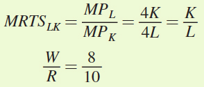
In Chapter 6, we learned that in the long run, a firm minimizes costs when it produces a quantity at which the marginal rate of technical substitution of labor for capital equals the ratio of the costs of labor (wage) and capital (rental rate): MRTSLK = W/R. We know that
To minimize costs, the firm will set MRTSLK = W/R:
To produce Q = 200 units, we can substitute for K in the production function and solve for L:
Q = 200 = 4KL = 4(0.8L)(L)
K = 0.8L = (0.8)(7.91) = 6.33
To minimize cost, the firm will want to increase labor from 5 to 7.91 units and reduce capital from 10 to 6.33 units. Total cost will fall to
TC = WL + RK = $8(7.91) + $10(6.33) = $63.28 + $63.30 = $126.58
Therefore, the firm will save $140 – $126.58 = $13.42.
Short-Run versus Long-Run Marginal Cost Curves
Just as the short- and long-run average total cost curves are related to the total cost curve, so are marginal costs over the two time horizons. Long-run marginal cost is the additional cost of producing another unit when inputs are fully flexible.
Every short-run average total cost curve has a corresponding short-run marginal cost curve that shows how costly it is to build another unit of output when capital is fixed at some particular level. A short-run marginal cost curve always crosses its corresponding short-run average total cost curve at the minimum of the average total cost curve.
While a long-run average total cost curve is the envelope of all the short-run average total cost curves, this isn’t true for short- and long-run marginal cost curves. Let’s look at the relationship between the two, step-by-step.
Figure 7.9 shows again the short- and long-run average total cost curves from Figure 7.8 and adds the short-run marginal cost curves corresponding to each short-run average total cost curve. (MCSR,10 is the short-run marginal cost for ATCSR,10, etc.)
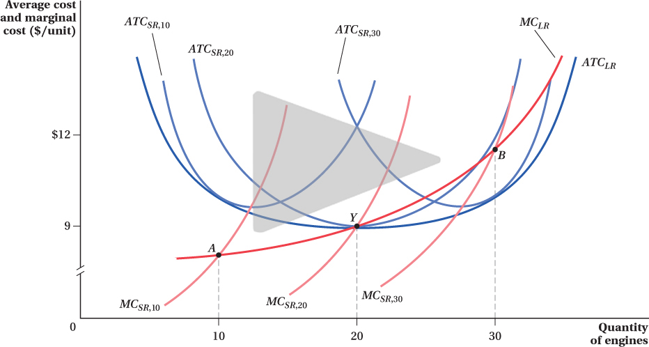
Figure 7.9: Figure 7.9 Long-Run and Short-Run Marginal Costs
Figure 7.9: MCSR,10, MCSR,20, and MCSR,30 are derived from ATCSR,10, ATCSR,20, and ATCSR,30, respectively. The long-run marginal cost curve must intersect MCSR,10, MCSR,20, and MCSR,30 at A, Y, and B, the points at which labor is cost-minimizing for Q = 10, Q = 20, and Q = 30 given
,
, and
. Therefore, A, Y, and B are the long-run marginal costs for Q = 10, Q = 20, and Q = 30, respectively, and the long-run marginal cost curve MCLR connects A, Y, and B.
How do we figure out what long-run marginal costs are? We know that in the short run with capital fixed, there is only one output level at which a firm would choose that same level of capital: the output at which the short-run average total cost curve touches the long-run average total cost curve. So, for example, if Q = 10, Ivor’s Engines would choose a level of capital in the long run (K = 4) that is the same as that corresponding to short-run average total cost curve ATCSR,10. Because the short- and long-run average total cost curves coincide at this quantity (but only at this quantity), so too do the short- and long-run marginal cost curves. In other words, because the firm would choose the same level of capital even if it were totally flexible, the long-run marginal cost at this quantity is the same as the short-run marginal cost on MCSR,10. Therefore, to find the long-run marginal cost of producing 10 units, we can go up to the short-run marginal cost curve at Q = 10. This is point A in Figure 7.9 and represents the long-run marginal cost at an output level of 10 engines.
Likewise, the long-run marginal cost at Q = 20 is the value of MCSR,20 when Ivor’s Engines is making 20 engines. Therefore, the long-run marginal cost at Q = 20 can be found at point Y in Figure 7.9 (this is the same point Y as in Figures 7.7 and 7.8). Repeating the logic, Ivor’s long-run marginal cost for producing 30 engines equals the value of MCSR,30 when output Q = 30, which is point B in the figure.
When we connect these long-run marginal cost points A, Y, and B, along with the similar points corresponding to every other output quantity, we trace out the long-run marginal cost curve MCLR. Notice that, just as we have discussed, long-run marginal cost is below long-run average total cost when average total cost is falling (such as at point A), above long-run average total cost when average total cost is rising (such as at point B), and equal to long-run average total cost when average total cost is at its minimum (point Y).
 See the problem worked out using calculus