nolanessentials3e

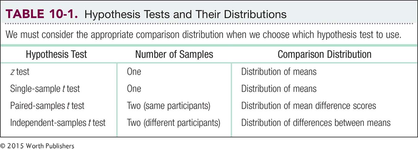
10.1 Conducting an Independent-Samples t Test

An independent-samples t test is used to compare two means for a between-groups design, a situation in which each participant is assigned to only one condition.

The independent-samples t test is used to compare two means for a between-groups design, a situation in which each participant is assigned to only one condition. This test uses a distribution of differences between means. This affects the t test in a few minor ways, most notably that it takes a bit more work when calculating a t test by hand (especially compared to using a computer!). The added calculation is that you have to estimate the appropriate standard error. It’s not difficult—just a bit time consuming.

Your Authors with Stella Cunliffe in 2010 In addition to her accomplishments as a statistician, Ms. Cunliffe was a leader of Britain’s Girl Guides, helped in relief work during WWII, and was the first civilian to enter the Bergen-Belsen concentration camp, an experience she recounted for the first time in a BBC interview in 2009.

ian.cunliffe1@nhs.net

A Distribution of Differences Between Means

MASTERING THE CONCEPT

10-1: An independent-samples t test is used when we have two groups and a between-groups research design—that is, every participant is in only one of the two groups.

Because we have different people in each condition of the study, we cannot create a difference score for each person. We’re looking at overall differences between two independent groups, so we need to develop a new type of distribution, a distribution of differences between means.

249

Let’s use the Chapter 6 data about heights to demonstrate how to create a distribution of differences between means. Let’s say that we were planning to collect data on two groups of three people each and wanted to determine the comparison distribution for this research scenario. Remember that in Chapter 6, we used the example of a population of 140 college students from the authors’ classes. We described writing the height of each student on a card and putting the 140 cards in a bowl.

EXAMPLE 10.1

Let’s use that example to create a distribution of differences between means. We’ll walk through the steps for this process.

STEP 1: We randomly select three cards, replacing each after selecting it, and calculate the mean of the heights listed on them. This is the first group.

STEP 2: We randomly select three other cards, replacing each after selecting it, and calculate their mean. This is the second group.

STEP 3: We subtract the second mean from the first.

That’s really all there is to it—except we repeat these three steps many more times. There are two samples, so there are two sample means, but we’re building just one distribution of differences between those means.

Here’s an example using the three steps.

STEP 1: We randomly select three cards, replacing each after selecting it, and find that the heights are 61, 65, and 72. We calculate a mean of 66 inches. This is the first group.

STEP 2: We randomly select three other cards, replacing each after selecting it, and find that the heights are 62, 65, and 65. We calculate a mean of 64 inches. This is the second group.

STEP 3: We subtract the second mean from the first: 66 − 64 = 2. (Note that it’s fine to subtract the first from the second, as long as we’re consistent in the arithmetic.)

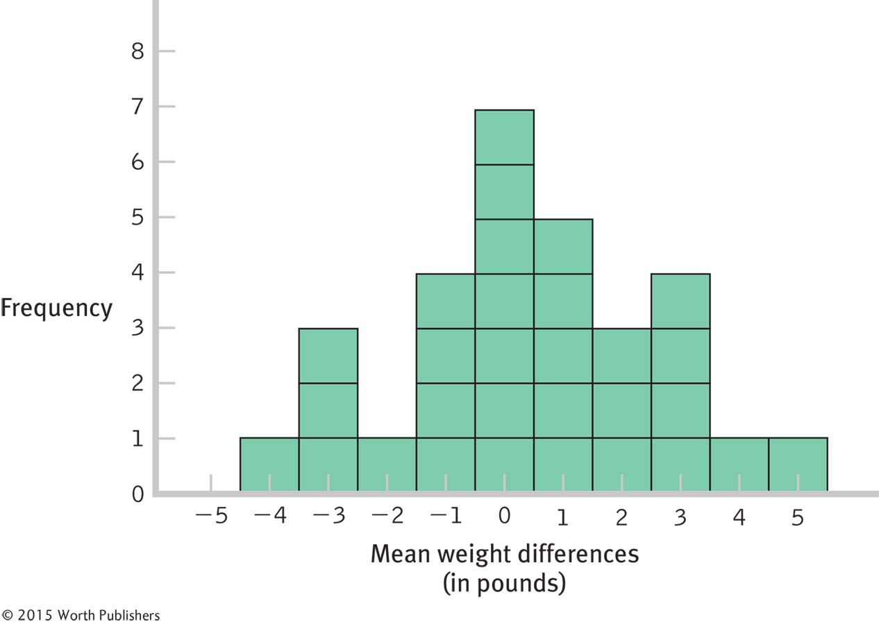
We repeat the three-step process. Let’s say that, this time, we calculate means of 65 and 68 for the two samples. Now the difference between means would be 65 − 68 = −3. We might repeat the three steps a third time and find means of 63 and 63, for a difference of 0. Eventually, we would have many differences between means—some positive, some negative, and some right at 0—and could plot them on a curve. But this would only be the beginning of what this distribution would look like. If we were to calculate the whole distribution, then we would do this many, many more times. When creating the beginning of a distribution of differences between means, the authors calculated 30 differences between means, as shown in Figure 10-1.

Figure 10.1: FIGURE 10-1
Distribution of Differences Between Means
This graph represents the beginning of the development of a distribution of differences between means. It includes only 30 differences, whereas the actual distribution would include all possible differences.

The Six Steps of the Independent-Samples t Test

250

EXAMPLE 10.2

Does the price of a product influence how much you like it? If you’re told that your sister’s new television cost $3000, do you perceive the picture quality to be sharper than if you’re told it cost $1200? If you think your friend’s new shirt is from a high-end designer like Dolce & Gabbana, do you covet it more than if he tells you it’s from a trendy but low-priced mass-retailer like Target?

Economics researchers from Northern California, not far from prime wine country, wondered whether enjoyment of wine is influenced by price (Plassmann, O’Doherty, Shiv, & Rangel, 2008). In part of their study, they randomly assigned some wine drinkers to taste wine that was said to cost $10 per bottle and others to taste the same wine at a supposed price of $90 per bottle. (Note that we’re altering some aspects of the design and statistical analysis of this study for teaching purposes, but the results are similar.) The researchers asked participants to rate how much they liked the wine; they also used functional magnetic resonance imaging (fMRI), a brain-scanning technique, to determine whether differences were evident in areas of the brain that are typically activated when people experience a stimulus as pleasant (e.g., the medial orbitofrontal cortex). Which do you think participants preferred, the wine priced at $10 or the same wine priced at $90?

We will conduct an independent-samples t test using the ratings of how much nine people like the wine they were randomly assigned to taste (four tasting wine from the “$10” bottle and five tasting wine from the “$90” bottle). Remember, everyone is actually tasting wine from the same bottle! Notice that we do not need to have the same number of participants in each sample, although it is best if the sample sizes are fairly similar.

Mean “liking ratings” of the wine

“$10” wine: 1.5 2.3 2.8 3.4

“$90” wine: 2.9 3.5 3.5 4.9 5.2

STEP 1: Identify the populations, distribution, and assumptions.

251

In terms of determining the populations, this step is similar to that for the paired-samples t test: There are two populations—those told they are drinking wine from a $10 bottle and those told they are drinking wine from a $90 bottle. The comparison distribution for an independent-samples t test, however, will be a distribution of differences between means (rather than a distribution of mean difference scores). Table 10-1 summarizes the distributions we have encountered with the hypothesis tests we have learned so far.

Price and Perception: Designer versus Knockoff Does the perceived price of a product influence how much you like it? The one on the right is the designer version. Quick—how much do you like it? OK, we lied; the one on the right is the knockoff. Did your perception of it change? If researchers ask some people to rate the designer version of Ray-Ban sunglasses and other people to rate the Ray-Ban knockoff version, we could conduct an independent-samples t test to determine if there is a statistically significant difference in the ratings.

As usual, the comparison distribution is based on the null hypothesis. As with the paired-samples t test, the null hypothesis for the independent-samples t test posits no mean difference. So the mean of the comparison distribution would be 0; this reflects a mean difference between means of 0. We compare the difference between the sample means to a difference of 0, which is what there would be if there were no difference between groups. The assumptions for an independent-samples t test are the same as those for the single-sample t test and the paired-samples t test.

Summary: Population 1: People told they are drinking wine from a $10 bottle. Population 2: People told they are drinking wine from a $90 bottle.

The comparison distribution will be a distribution of differences between means based on the null hypothesis. The hypothesis test will be an independent-samples t test because we have two samples composed of different groups of participants. This study meets one of the three assumptions. (1) The dependent variable is a rating on a liking measure, which can be considered a scale variable. (2) We do not know whether the population is normally distributed, and there are not at least 30 participants. However, the sample data do not suggest that the underlying population distribution is skewed. (3) The wine drinkers in this study were not randomly selected from among all wine drinkers, so we must be cautious with respect to generalizing these findings.

252

STEP 2: State the null and research hypotheses.

This step for an independent-samples t test is identical to that for the previous t tests.

Summary: Null hypothesis: On average, people drinking wine they were told was from a $10 bottle give it the same rating as do people drinking wine they were told was from a $90 bottle—H₀: μ₁ = μ₂. Research hypothesis: On average, people drinking wine they were told was from a $10 bottle give it a different rating than do people drinking wine they were told was from a $90 bottle—H₁: μ₁ ≠ μ₂.

STEP 3: Determine the characteristics of the comparison distribution.

This step for an independent-samples t test is similar to that for previous t tests: We determine the appropriate mean and the appropriate standard error of the comparison distribution—the distribution based on the null hypothesis. According to the null hypothesis, no mean difference exists between the populations; that is, the difference between means is 0. So the mean of the comparison distribution is always 0, as long as the null hypothesis posits no mean difference.

Because we have two samples for an independent-samples t test, however, it is more complicated to calculate the appropriate measure of spread. There are five stages to this process. First, let’s consider them in words; then we’ll learn the calculations. These instructions are basic, and you’ll understand them better when you do the calculations, but they’ll help you to keep the overall framework in mind. (These verbal descriptions are keyed by letter to the calculation stages below.)

Calculate the corrected variance for each sample. (Notice that we’re working with variance, not standard deviation.)
Pool the variances. Pooling the variances involves taking an average of the two sample variances while accounting for any differences in the sizes of the two samples. Pooled variance is an estimate of the common population variance.
Convert the pooled variance from squared standard deviation (that is, variance) to squared standard error (another version of variance) by dividing the pooled variance by the sample size, first for one sample and then again for the second sample. These are the estimated variances for each sample’s distribution of means.
Add the two variances (squared standard errors), one for each distribution of sample means, to calculate the estimated variance of the distribution of differences between means.
Calculate the square root of this form of variance (squared standard error) to get the estimated standard error of the distribution of differences between means.

Notice that stages (a) and (b) are an expanded version of the usual first calculation for a t test. Instead of calculating one corrected estimate of standard deviation, we’re calculating two for an independent-samples t test—one for each sample. Also, for an independent-samples t test, we use variances instead of standard deviations. Because there are two calculations of variance, we combine them (i.e., the pooled variance). Stages (c) and (d) are an expanded version of the usual second calculation for a t test. Once again, we convert to standard error for each sample (only this time it is squared because we are working with variances) and combine the variances from each sample. In stage (e), we take the square root so that we have standard error. Let’s examine the calculations.

253

We calculate corrected variance for each sample (corrected variance is the one we learned in Chapter 9 that uses N − 1 in the denominator). First, we calculate variance for X, the sample of people told they are drinking wine from a $10 bottle. Be sure to use the mean of the ratings of the $10 wine drinkers only, which we calculate to be 2.5. Notice that the symbol for this variance uses s², instead of SD² (just as the standard deviation used s instead of SD in the previous t tests). Also, we included the subscript X to indicate that this is variance for the first sample, whose scores are arbitrarily called X. (Remember, don’t take the square root. We want variance, not standard deviation.)

X X − M (X − M)²

1.5 −1.0 1.00

2.3 −0.2 0.04

2.8 0.3 0.09

3.4 0.9 0.81

Now we do the same for Y, the people told they are drinking wine from a $90 bottle. Remember to use the mean for Y; it’s easy to forget and use the mean we calculated earlier for X. We calculate the mean for Y to be 4.0. The subscript Y indicates that this is the variance for the second sample, whose scores are arbitrarily called Y. (We could call these scores by any letter, but statisticians tend to call the scores in the first two samples X and Y.)

Y	Y − M	(Y − M)²
2.9	−1.1	1.21
3.5	−0.5	0.25
3.5	−0.5	0.25
4.9	0.9	0.81
5.2	1.2	1.44

MASTERING THE FORMULA

10-1: There are three degrees of freedom calculations for an independent-samples t test. We calculate the degrees of freedom for each sample by subtracting 1 from the number of participants in that sample: df_X = N − 1 and df_Y = N − 1. Finally, we sum the degrees of freedom from the two samples to calculate the total degrees of freedom: df_total = df_X + df_Y.

We pool the two estimates of variance. Because there are often different numbers of people in each sample, we cannot simply take their mean. We mentioned earlier in this book that estimates of spread taken from smaller samples tend to be less accurate. So we weight the estimate from the smaller sample a bit less and weight the estimate from the larger sample a bit more. We do this by calculating the proportion of degrees of freedom represented by each sample. Each sample has degrees of freedom of N − 1. We also calculate a total degrees of freedom that sums the degrees of freedom for the two samples. Here are the calculations:

254

df_X = N − 1 = 4 − 1 = 3

df_Y = N − 1 = 5 − 1 = 4

df_total = df_X + df_Y = 3 + 4 = 7

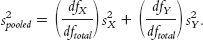
Pooled variance is a weighted average of the two estimates of variance—one from each sample—that are calculated when conducting an independent-samples t test.

MASTERING THE FORMULA

10-2: We use all three degrees of freedom calculations, along with the variance estimates for each sample, to calculate pooled variance:

This formula takes into account the size of each sample. A larger sample has more degrees of freedom in the numerator, and that variance therefore has more weight in the pooled variance calculations.

Using these degrees of freedom, we calculate a sort of average variance. Pooled variance is a weighted average of the two estimates of variance—one from each sample—that are calculated when conducting an independent-samples t test. The estimate of variance from the larger sample counts for more in the pooled variance than does the estimate from the smaller sample because larger samples tend to lead to somewhat more accurate estimates than do smaller samples. Here’s the formula for pooled variance, and the calculations for this example:

(Note: If we had exactly the same number of participants in each sample, this would be an unweighted average—that is, we could compute the average in the usual way by summing the two sample variances and dividing by 2.)

MASTERING THE FORMULA

10-3: The next step in calculating the t statistic for a two-sample, between-groups design is to calculate the variance version of standard error for each sample by dividing variance by sample size. We use the pooled version of variance for both calculations. For the first sample, the formula is:

For the second sample, the formula is:

Note that because we’re dealing with variance, the square of standard deviation, we divide by N, the square of —the denominator for standard error.

Now that we have pooled the variances, we have an estimate of spread. This is similar to the estimate of the standard deviation in the previous t tests, but now it’s based on two samples (and is an estimate of variance rather than standard deviation). The next calculation in the previous t tests was dividing standard deviation by to get standard error. In this case, we divide by N instead of . Why? Because we are dealing with variances, not standard deviations. Variance is the square of standard deviation, so we divide by the square of , which is simply N. We do this once for each sample, using pooled variance as the estimate of spread. We use pooled variance because an estimate based on two samples is better than an estimate based on one. The key here is to divide by the appropriate N: in this case, 4 for the first sample and 5 for the second sample.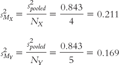
In stage (c), we calculated the variance versions of standard error for each sample, but we want only one such measure of spread when we calculate the test statistic. So, we combine the two variances, similar to the way in which we combined the two estimates of variance in stage (b). This stage is even simpler, however. We merely add the two variances together. When we sum them, we get the variance of the distribution of differences between means, symbolized as s²_difference. Here are the formula and the calculations for this example:

MASTERING THE FORMULA

10-4: To calculate the variance of the distribution of differences between means, we sum the variance versions of standard error that we calculated in the previous step:

s²_difference = s²_MX + s²_MY

s²_difference = s²_MX + s²_MY = 0.211 + 0.169 = 0.380
We now have paralleled the two calculations of the previous t tests by doing two things: (1) We calculated an estimate of spread (we made two calculations, one for each sample, then combined them), and (2) we then adjusted the estimate for the sample size (again, we made two calculations, one for each sample, then combined them). The main difference is that we have kept all calculations as variances rather than standard deviations. At this final stage, we convert from variance form to standard deviation form. Because standard deviation is the square root of variance, we do this by simply taking the square root:

255

MASTERING THE FORMULA

10-5: To calculate the standard deviation of the distribution of differences between means, we take the square root of the previous calculation, the variance of the distribution of differences between means. The formula is: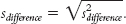

Summary: The mean of the distribution of differences between means is: μ_X − μ_Y = 0. The standard deviation of the distribution of differences between means is: s_difference = 0.616.

STEP 4: Determine critical values, or cutoffs.

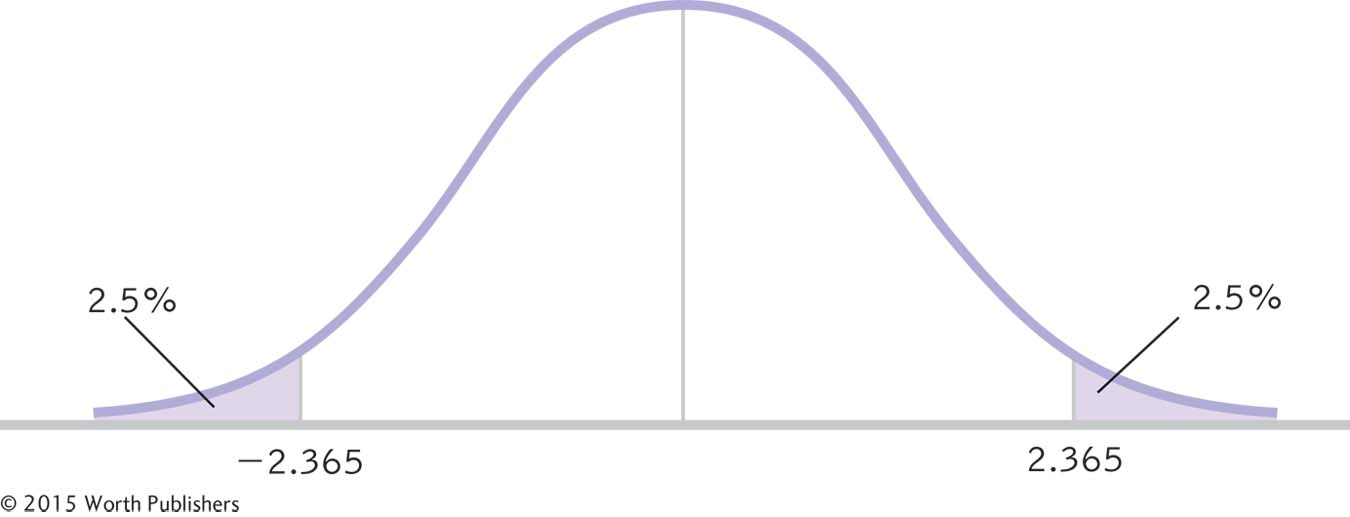
This step for the independent-samples t test is similar to those for previous t tests, but we use the total degrees of freedom, df_total.

Summary: The critical values, based on a two-tailed test, a p level of 0.05, and a df_total of 7, are −2.365 and 2.365 (as seen in the curve in Figure 10-2).

Figure 10.3: FIGURE 10-2
Determining Cutoffs for an Independent-Samples t Test
To determine the critical values for an independent-samples t test, we use the total degrees of freedom, df_total. This is the sum of the degrees of freedom for each sample, which is N − 1 for each sample.

STEP 5: Calculate the test statistic.

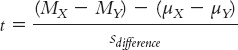
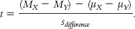
This step for the independent-samples t test is similar to the fifth step in previous t tests. Here we subtract the population difference between means based on the null hypothesis from the difference between means for the samples. The formula is:

As in previous t tests, the test statistic is calculated by subtracting a number based on the populations from a number based on the samples, then dividing by a version of standard error. Because the population difference between means (according to the null hypothesis) is almost always 0, many statisticians choose to eliminate the latter part of the formula. 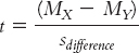So the formula for the test statistic for an independent-samples t test is often abbreviated as:

256

You might find it easier to use the first formula, however, as it reminds us that we are subtracting the population difference between means according to the null hypothesis (0) from the actual difference between the sample means. This format more closely parallels the formulas of the test statistics we calculated in Chapter 9.

MASTERING THE FORMULA

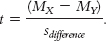
10-6: We calculate the test statistic for an independent-samples t test using the following formula:

We subtract the difference between means according to the null hypothesis, usually 0, from the difference between means in the sample. We then divide this by the standard deviation of the differences between means. Because the difference between means according to the null hypothesis is usually 0, the formula for the test statistic is often abbreviated as:

Summary: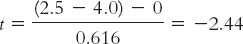

STEP 6: Make a decision.

This step for the independent-samples t test is identical to that for the previous t tests. If we reject the null hypothesis, we need to examine the means of the two conditions so that we know the direction of the effect.

Summary: Reject the null hypothesis. It appears that those told they are drinking wine from a $10 bottle give it lower ratings, on average, than those told they are drinking from a $90 bottle (as shown by the curve in Figure 10-3).

Figure 10.4: FIGURE 10-3
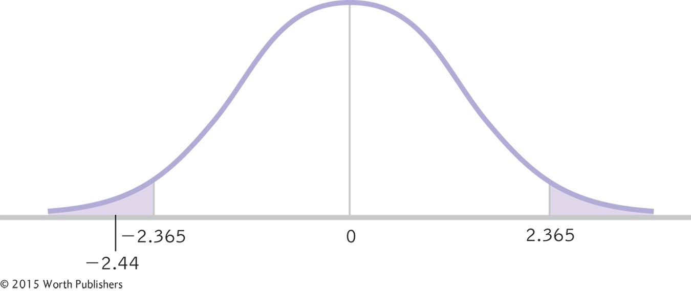
Making a Decision
As in previous t tests, in order to decide whether or not to reject the null hypothesis, we compare the test statistic to the critical values. In this figure, the test statistic, −2.44, is beyond the lower cutoff, −2.365. We reject the null hypothesis. It appears that those told they are drinking wine from a $10 bottle give it lower ratings, on average, than those told they are drinking wine from a $90 bottle.

This finding documents the fact that people report liking a more expensive wine better than a less expensive one—even when it’s the same wine! The researchers documented a similar finding with a narrower gap between prices—$5 and $45. Naysayers might point out, however, that participants drinking an expensive wine may report liking it better than participants drinking an inexpensive wine simply because they are expected to say they like it better because of its price. However, the fMRI that was conducted, which is a more objective measure, yielded a similar finding. Those drinking the supposedly more expensive wines showed increased activation in brain areas such as the medial orbitofrontal cortex, essentially an indication in the brain that people are enjoying an experience. Expectations really do seem to influence us.

Reporting the Statistics

To report the statistics as they would appear in a journal article, follow standard APA format. Be sure to include the degrees of freedom, the value of the test statistic, and the p value associated with the test statistic. (Note that because the t table in Appendix B only includes the p values of 0.10, 0.05, and 0.01, we cannot use it to determine the actual p value for the test statistic. Unless we use software, we can only report whether or not the p value is less than the critical p level.) In the current example, the statistics would read:

t(7) = −2.44, p < 0.05

257

In addition to the results of hypothesis testing, we would also include the means and standard deviations for the two samples. We calculated the means in step 3 of hypothesis testing, and we also calculated the variances (0.647 for those told they were drinking from a $10 bottle and 0.990 for those told they were drinking from a $90 bottle). We can calculate the standard deviations by taking the square roots of the variances. The descriptive statistics can be reported in parentheses as:

($10 bottle: M = 2.5, SD = 0.80; $90 bottle: M = 4.0, SD = 0.99)

CHECK YOUR LEARNING

Reviewing the Concepts		When we conduct an independent-samples t test, we cannot calculate individual difference scores. That is why we compare the mean of one sample with the mean of the other sample. The comparison distribution is a distribution of differences between means. We use the same six steps of hypothesis testing that we used with the z test and with the single-sample and paired-samples t tests. Conceptually, the t test for independent samples makes the same comparisons as the other t tests. However, the calculations are different, and critical values are based on degrees of freedom from two samples.
Clarifying the Concepts	10-1	In what situation do we conduct a paired-samples t test? In what situation do we conduct an independent-samples t test?
	10-2	What is pooled variance?
Calculating the Statistics	10-3	Imagine you have the following data from two independent groups: Group 1: 3, 2, 4, 6, 1, 2 Group 2: 5, 4, 6, 2, 6 Compute each of the following calculations needed to complete your final calculation of the independent-samples t test. Calculate the corrected variance for each group. Calculate the degrees of freedom and pooled variance. Calculate the variance version of standard error for each group. Calculate the variance of the distribution of differences between means, then convert this number to standard deviation. Calculate the test statistic.
Applying the Concepts	10-4	In Check Your Learning 10-3, you calculated several statistics; now let’s consider a context for those numbers. Steele and Pinto (2006) examined whether people’s level of trust in their direct supervisor was related to their level of agreement with a policy supported by that leader. They found that the extent to which subordinates agreed with their supervisor was statistically significantly related to trust and showed no relation to gender, age, time on the job, or length of time working with the supervisor. We have presented fictional data to re-create these findings, where group 1 represents employees with low trust in their supervisor and group 2 represents the high-trust employees. The scores presented are the level of agreement with a decision made by a leader, from 1 (strongly disagree) to 7 (strongly agree). Group 1 (low trust in leader): 3, 2, 4, 6, 1, 2 Group 2 (high trust in leader): 5, 4, 6, 2, 6 State the null and research hypotheses. Identify the critical values and make a decision. Write your conclusion in a formal sentence that includes presentation of the statistic in APA format. Explain why your results are different from those in the original research, despite having a similar mean difference.

Solutions to these Check Your Learning questions can be found in Appendix D.

X	X − M	(X − M)²
1.5	−1.0	1.00
2.3	−0.2	0.04
2.8	0.3	0.09
3.4	0.9	0.81