10.2 Beyond Hypothesis Testing
MASTERING THE CONCEPT
10-
After working at Guinness, Stella Cunliffe was hired by the British government’s criminology department. She noticed that adult male prisoners who had short prison sentences returned to prison at a very high rate—
Two ways that researchers can evaluate the findings of a hypothesis test are by calculating a confidence interval and an effect size.
Calculating a Confidence Interval for an Independent-Samples t Test
Confidence intervals for the independent-
We use the formula for the independent-
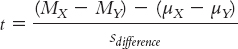
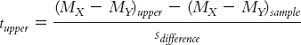
We replace the population mean difference, (μX − μY), with the sample mean difference (MX − MY)sample, because this is what the confidence interval is centered around. We also indicate that the first mean difference in the numerator refers to the bounds of the confidence intervals, the upper bound in this case:
MASTERING THE FORMULA
10-
With algebra, we isolate the upper bound of the confidence interval to create the following formula:
(MX − MY)upper = t(sdifference) + (MX − MY)sample
We create the formula for the lower bound of the confidence interval in exactly the same way, using the negative version of the t statistic:
(MX − MY)lower = −t(sdifference) + (MX − MY)sample
EXAMPLE 10.3
Let’s calculate the confidence interval that parallels the hypothesis test we conducted earlier, comparing ratings of those who are told they are drinking wine from a $10 bottle and ratings of those told they are drinking wine from a $90 bottle (Plassmann et al., 2008). The difference between the means of these samples was calculated in the numerator of the t statistic. It is 2.5 − 4.0 = −1.5. (Note that the order of subtraction in calculating the difference between means is irrelevant; we could just as easily have subtracted 2.5 from 4.0 and gotten a positive result, 1.5.) The standard error for the differences between means, sdifference, was calculated to be 0.616. The degrees of freedom were determined to be 7. Here are the five steps for determining a confidence interval for a difference between means:
STEP 1: Draw a normal curve with the sample difference between means in the center (as shown in Figure 10-4).
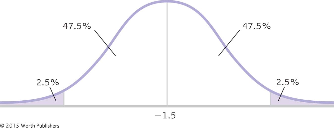
A 95% Confidence Interval for Differences Between Means, Part I
As with a confidence interval for a single-
STEP 2: Indicate the bounds of the confidence interval on either end, and write the percentages under each segment of the curve (see Figure 10-4).
STEP 3: Look up the t statistics for the lower and upper ends of the confidence interval in the t table.
Use a two-
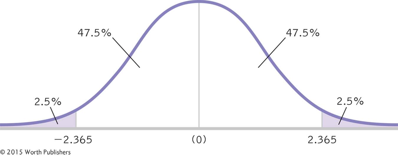
A 95% Confidence Interval for Differences Between Means, Part II
The next step in calculating a confidence interval is identifying the t statistics that indicate each end of the interval. Because the curve is symmetric, the t statistics have the same magnitude—
STEP 4: Convert the t statistics to raw differences between means for the lower and upper ends of the confidence interval.
For the lower end, the formula is:
(MX − MY)lower = −t(sdifference) + (MX − MY)sample
= −2.365(0.616) + (−1.5) = −2.96
For the upper end, the formula is:
(MX − MY)upper = t(sdifference) + (MX − MY)sample
= 2.365(0.616) + (−1.5) = −0.04
confidence interval is [−2.96, −0.04], as shown in Figure 10-6.
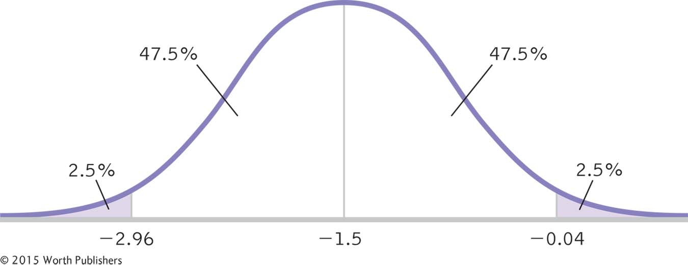
A 95% Confidence Interval for Differences Between Means, Part III
The final step in calculating a confidence interval is converting the t statistics that indicate each end of the interval into raw differences between means.
STEP 5: Check your answer
Each end of the confidence interval should be exactly the same distance from the sample mean.
−2.96 − (−1.5) = −1.46
−0.04 − (−1.5) = 1.46
The interval checks out. The bounds of the confidence interval are calculated as the difference between sample means, plus or minus 1.46. Also, the confidence interval does not include 0; thus, it is not plausible that there is no difference between means. We can conclude that people told they are drinking wine from a $10 bottle give different ratings, on average, than those told they are drinking wine from a $90 bottle. When we conducted the independent-
Calculating Effect Size for an Independent-Samples t Test
EXAMPLE 10.4
As with all hypothesis tests, it is recommended that the results be supplemented with an effect size. For an independent-
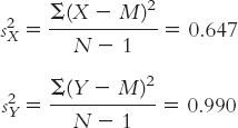
Stage (a) (variance for each sample):
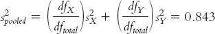
Stage (b) (combining variances):
Stage (c) (variance form of standard error for each sample):
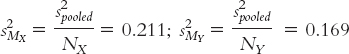
Stage (d) (combining variance forms of standard error):
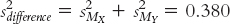
Stage (e) (converting the variance form of standard error to the standard deviation form of standard error):
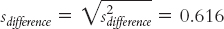
Because the goal is to disregard the influence of sample size in order to calculate Cohen’s d, we want to use the standard deviation, rather than the standard error, in the denominator. So we can ignore the last three stages, all of which contribute to the calculation of standard error. That leaves stages (a) and (b). It makes more sense to use the one that includes information from both samples, so we focus our attention on stage (b). Here is where many students make a mistake. What we have calculated in stage (b) is pooled variance, not pooled standard deviation. We must take the square root of the pooled variance to get the pooled standard deviation, the appropriate value for the denominator of Cohen’s d.

The test statistic that we calculated for this study was:
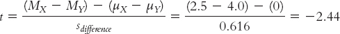
For Cohen’s d, we simply replace the denominator with standard deviation, spooled, instead of standard error, sdifference.

MASTERING THE FORMULA
10-
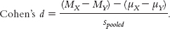
The formula is similar to that for the test statistic in an independent-
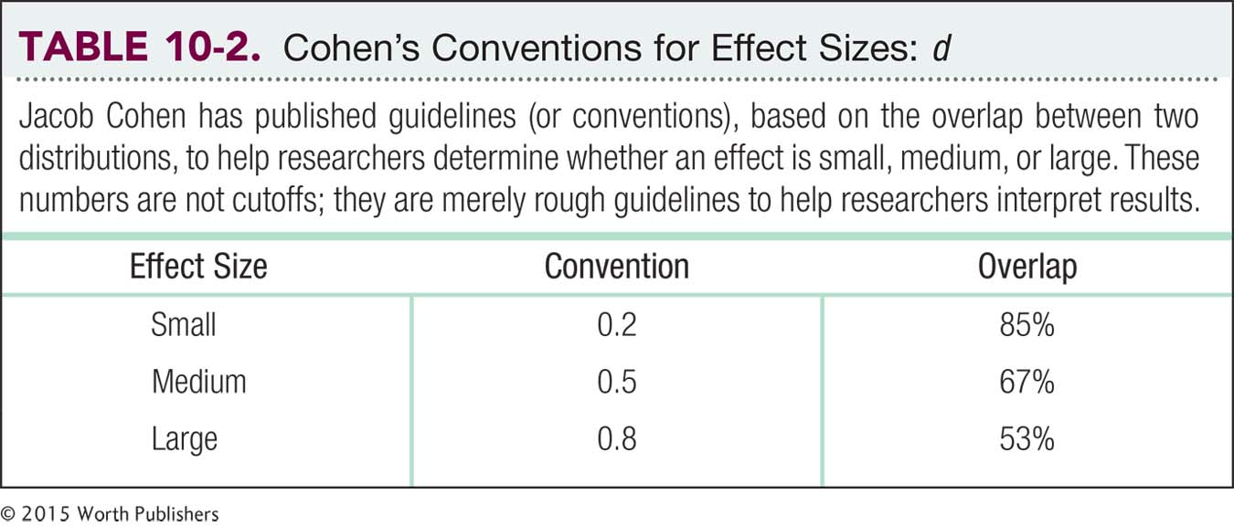
For this study, the effect size is reported as: d = 1.63. The two sample means are 1.63 standard deviations apart. According to the conventions that we learned in Chapter 8 and are shown again in Table 10-2, this is a large effect.
CHECK YOUR LEARNING
| Reviewing the Concepts |
|
|
| Clarifying the Concepts | 10- |
Why do we calculate confidence intervals? |
| 10- |
How does considering the conclusions in terms of effect size help to prevent incorrect interpretations of the findings? | |
| Calculating the Statistics | 10- |
Use the hypothetical data on level of agreement with a supervisor, as listed here, to calculate the following. We already made some of these calculations for Check Your Learning 10- Group 1 (low trust in leader): 3, 2, 4, 6, 1, 2 Group 2 (high trust in leader): 5, 4, 6, 2, 6
|
| Applying the Concepts | 10- |
Explain what the confidence interval calculated in Check Your Learning 10- |
| 10- |
Interpret the meaning of the effect size calculated in Check Your Learning 10- |
Solutions to these Check Your Learning questions can be found in Appendix D.