12.3 Conducting a Two-Way Between-Groups ANOVA
Understanding interactions makes it easier to explain patterns in the data. For example, it is easy to understand why a ski resort would be tempted to exaggerate snowfall reports—
Behavioral scientists explore interactions by using two-
The three ideas being tested in a two-
The Six Steps of Two-Way ANOVA
Two-
EXAMPLE 12.4
Does myth busting really improve public health? Here are some myths and facts.
From the Web site of the Canadian Mental Health Association (2015):
Myth: “People who experience mental illnesses can’t work.”
Fact: “Whether you realize it or not, workplaces are filled with people who have experienced mental illnesses. Mental illnesses don’t mean that someone is no longer capable of working.”
From the Web site for the World Health Organization (2015):
Myth: “Disasters bring out the worst in human behavior.”
Fact: “Although isolated cases of antisocial behavior exist, the majority of people respond spontaneously and generously.”
A group of Canadian researchers examined the effectiveness of myth busting (Skurnik, Yoon, Park, & Schwarz, 2005). They wondered whether the effectiveness of debunking false medical claims depends on the age of the person targeted by the message. In one study, they compared two groups of adults: younger adults, ages 18–
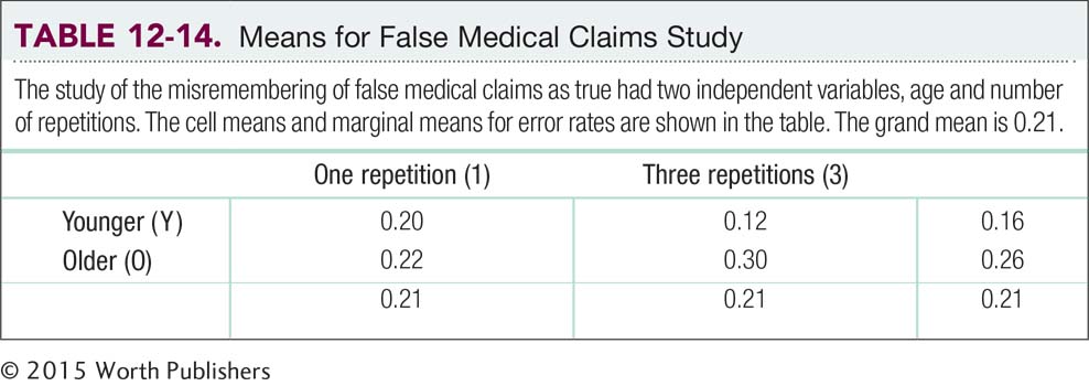
The two independent variables in this study were age, with two levels (younger, older), and number of repetitions, with two levels (once, three times). The dependent variable, proportion of responses that were wrong after a 3-
| Experimental Conditions | Proportion of Responses That Were Wrong | Mean |
| Younger, one repetition | 0.25, 0.21, 0.14 | 0.20 |
| Younger, three repetitions | 0.07, 0.13, 0.16 | 0.12 |
| Older, one repetition | 0.27, 0.22, 0.17 | 0.22 |
| Older, three repetitions | 0.33, 0.31, 0.26 | 0.30 |
Let’s consider the steps of hypothesis testing for a two-
STEP 1: Identify the populations, distribution, and assumptions.
The first step of hypothesis testing for a two-
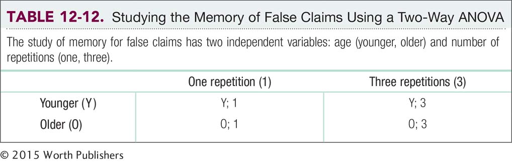
There are four populations, each with labels representing the levels of the two independent variables to which they belong.
Population 1 (Y; 1): Younger adults who hear one repetition of a false claim
Population 2 (Y; 3): Younger adults who hear three repetitions of a false claim
Population 3 (O; 1): Older adults who hear one repetition of a false claim
Population 4 (O; 3): Older adults who hear three repetitions of a false claim
We next consider the characteristics of the data to determine the distributions to which we compare the sample. We have more than two groups, so we need to consider variances to analyze differences among means. Therefore, we use F distributions. Finally, we list the hypothesis test that we use for those distributions and check the assumptions for that test. For F distributions, we use ANOVA—
The assumptions are the same for all types of ANOVA: The sample should be selected randomly; the populations should be distributed normally; and the population variances should be equal. Let’s explore that a bit further.
(1) These data were not randomly selected. Younger adults were recruited from a university, and older adults were recruited from the local community. Because random sampling was not used, we must be cautious when generalizing from these samples. (2) The researchers did not report whether they investigated the shapes of the distributions of their samples to assess the shapes of the underlying populations. (3) The researchers did not provide standard deviations of the samples as an indication of whether the population spreads might be approximately equal—
Summary: Population 1 (Y; 1): Younger adults who hear one repetition of a false claim. Population 2 (Y; 3): Younger adults who hear three repetitions of a false claim. Population 3 (O; 1): Older adults who hear one repetition of a false claim. Population 4 (O; 3): Older adults who hear three repetitions of a false claim.
The comparison distributions will be F distributions. The hypothesis test will be a two-
STEP 2: State the null and research hypotheses.
The second step, to state the null and research hypotheses, is similar to that for a one-
The hypotheses for the interaction are typically stated in words but not in symbols. The null hypothesis is that the effect of one independent variable is not dependent on the levels of the other independent variable. The research hypothesis is that the effect of one independent variable depends on the levels of the other independent variable. It does not matter which independent variable we list first (e.g., “The effect of age is not dependent. . .” or “The effect of number of repetitions is not dependent. . .”). Write the hypotheses in the way that makes the most sense to you.
Summary: The hypotheses for the main effect of the first independent variable, age, are as follows. Null hypothesis: On average, compared with older adults, younger adults have the same proportion of responses that are wrong when remembering which claims are myths—
The hypotheses for the main effect of the second independent variable, number of repetitions, are as follows. Null hypothesis: On average, those who hear one repetition have the same proportion of responses that are wrong when remembering which claims are myths compared with those who hear three repetitions—
The hypotheses for the interaction of age and number of repetitions are as follows. Null hypothesis: The effect of number of repetitions is not dependent on the levels of age. Research hypothesis: The effect of number of repetitions depends on the levels of age.
STEP 3: Determine the characteristics of the comparison distribution.
The third step is similar to that of a one-
MASTERING THE FORMULA
12-
dfrows = Nrows – 1.
We subtract 1 from the number of rows, representing levels, for that variable.
For each main effect, the between-
dfrows(age) = Nrows − 1 = 2 − 1 = 1
MASTERING THE FORMULA
12-
dfcolumns = Ncolumns – 1.
We subtract 1 from the number of columns, representing levels, for that variable.
The second independent variable, number of repetitions, is in the columns of the table of cells, so the between-
dfcolumns(reps) = Ncolumns − 1 = 2 − 1 = 1
MASTERING THE FORMULA
12-
dfinteraction = (dfrows)(dfcolumns).
We multiply the degrees of freedom for each of the independent variables.
We now need a between-
dfinteraction = (dfrows(age))(dfcolumns(reps)) = (1)(1) = 1
The within-
dfY,1 = N − 1 = 3 − 1 = 2
dfY,3 = N − 1 = 3 − 1 = 2
dfO,1 = N − 1 = 3 − 1 = 2
dfO,3 = N − 1 = 3 − 1 = 2
dfwithin = dfY,1 + dfY,3 + dfO,1 + dfO,3 = 2 + 2 + 2 + 2 = 8
MASTERING THE FORMULA
12-
dfwithin = dfcell 1 + dfcell 2 + dfcell 3 + dfcell 4.
For a check on our work, we calculate the total degrees of freedom just as we did for the one-
dftotal = Ntotal − 1 = 12 − 1 = 11
We now add up the three between-
11 = 1 + 1 + 1 +8
MASTERING THE FORMULA
12-
dftotal = Ntotal − 1.
We can also add the three between-
Finally, for this step, we list the distributions with their degrees of freedom for the three effects. Note that, although the between-
Summary: Main effect of age: F distribution with 1 and 8 degrees of freedom. Main effect of number of repetitions: F distribution with 1 and 8 degrees of freedom. Interaction of age and number of repetitions: F distribution with 1 and 8 degrees of freedom. (Note: It is helpful to include all degrees of freedom calculations in this step.)
STEP 4: Determine the critical values, or cutoffs.
Again, this step for the two-
For each main effect and for the interaction, we look up the within-
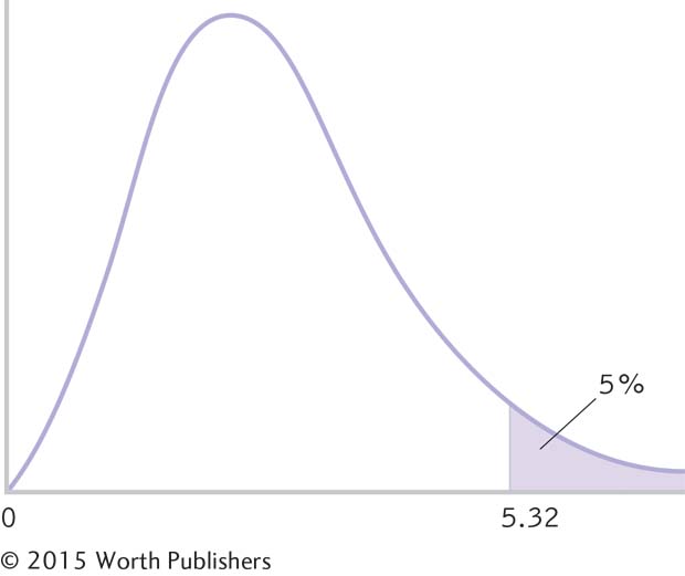
Determining Cutoffs for an F Distribution
We determine the critical values for an F distribution for a two-
Summary: There are three critical values (which in this case are all the same), as seen in the curve in Figure 12-8. The critical F value for the main effect of age is 5.32. The critical F value for the main effect of number of repetitions is 5.32. The critical F value for the interaction of age and number of repetitions is 5.32.
STEP 5: Calculate the test statistic.
As with the one-
STEP 6: Make a decision.
This step is the same as for a one-
First, if we are able to reject the null hypothesis for the interaction, then we draw a specific conclusion with the help of a table and graph. Because we have more than two groups, we use a post hoc test, such as the one that we learned in Chapter 11. When there are three effects, post hoc tests are typically implemented separately for each main effect and for the interaction (Hays, 1994). If the interaction is statistically significant, then it might not matter whether the main effects are also significant; if they are also significant, then those findings are usually qualified by the interaction, and are not described separately. The overall pattern of cell means tells the whole story.
Second, if we are not able to reject the null hypothesis for the interaction, then we focus on any significant main effects, drawing a specific directional conclusion for each. In this study, each independent variable has only two levels, so there is no need for a post hoc test. If there were three or more levels, however, then each significant main effect would require a post hoc test to determine exactly where the differences lie.
Third, if we do not reject the null hypothesis for either main effect or the interaction, then we can only conclude that there is insufficient evidence from this study to support the research hypotheses. We will complete step 6 of hypothesis testing for this study in the next section, after we consider the calculations of the source table for a two-
Identifying Four Sources of Variability in a Two-Way ANOVA
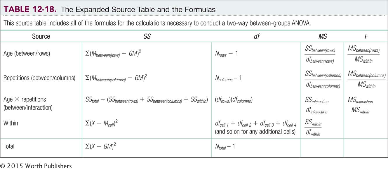
In this section, we complete step 5 for a two-
MASTERING THE FORMULA
12-
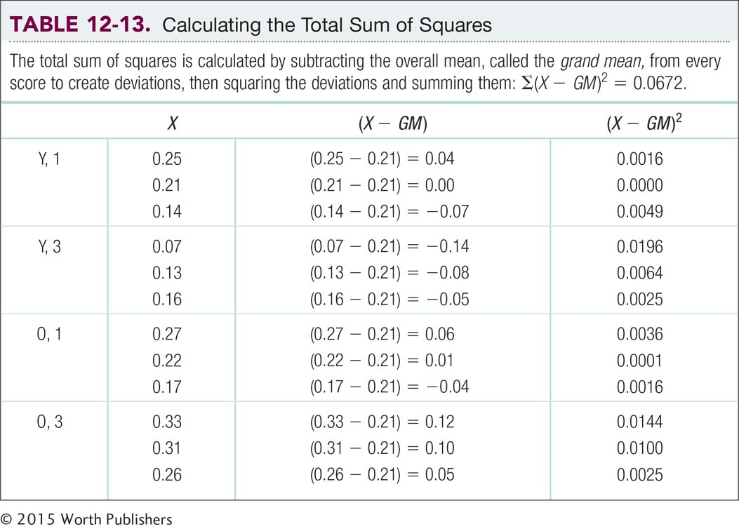
SStotal =∑(X − GM )2.
We subtract the grand mean from every score to create deviations, then square the deviations, and finally sum the squared deviations.
First, we calculate the total sum of squares (Table 12-13). We calculate this number in exactly the same way as we do for a one-
SStotal = ∑(X − GM )2 = 0.0672
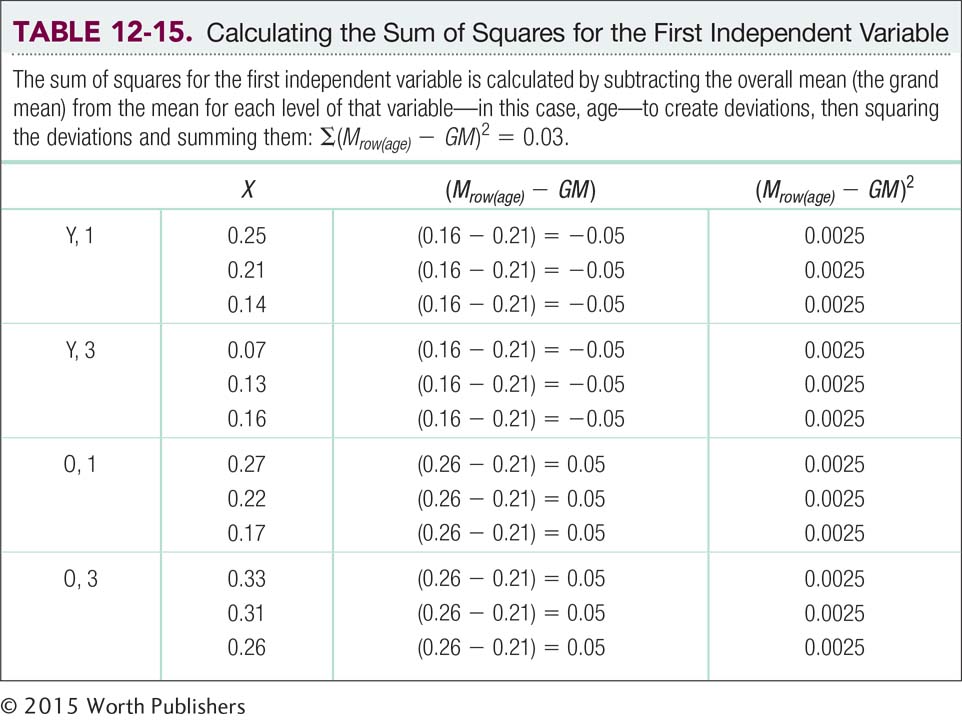
We now calculate the between-
MASTERING THE FORMULA
12-
SSbetween(rows) =∑(Mrow − GM )2.
For every participant, we subtract the grand mean from the marginal mean for the appropriate row for that participant. We square these deviations, and sum the squared deviations.
SSbetween(rows) =∑(Mrow(age) − GM )2 = 0.03
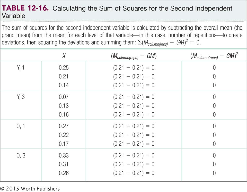
We repeat this process for the second possible main effect, that of the independent variable in the columns (Table 12-16). The between-
MASTERING THE FORMULA
12-
SSbetween(columns) =∑(Mcolumn − GM )2.
For every participant, we subtract the grand mean from the marginal mean for the appropriate column for that participant. We square these deviations, and then sum the squared deviations.
SSbetween(columns) =∑(Mcolumns(reps) − GM )2 = 0
The within-
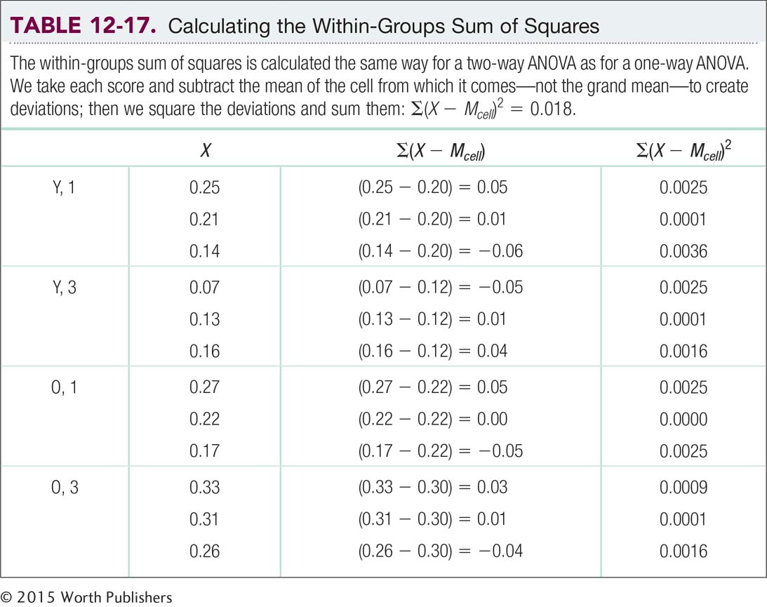
SSwithin = ∑(X − Mcell)2 = 0.018
MASTERING THE FORMULA
12-
SSwithin =?∑(X − Mcell)2.
For every participant, we subtract the appropriate cell mean from that participant’s score. We square these deviations, and sum the squared deviations.
All we need now is the between-
SSbetween(interaction) = SStotal − (SSbetween(rows) + SSbetween(columns) + SSwithin)
The calculations are:
SSbetween(interaction) = 0.0672 − (0.03 + 0 + 0.018) = 0.0192
MASTERING THE FORMULA
12-
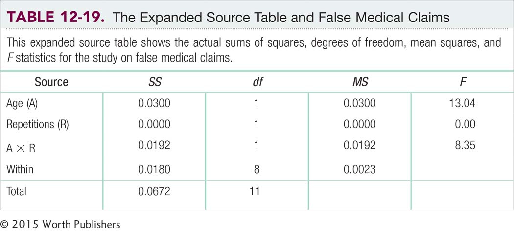
Now we complete step 6 of hypothesis testing by calculating the F statistics using the formulas in Table 12-18. The results are in the source table (Table 12-19). The main effect of age is statistically significant because the F statistic, 13.04, is larger than the critical value of 5.32. The means tell us that older participants tend to make more mistakes, remembering more medical myths as true, than do younger participants. The main effect of number of repetitions is not statistically significant, however, because the F statistic of 0.00 is not larger than the cutoff of 5.32. It is unusual to have an F statistic of 0.00. Even when there is no statistically significant effect, there is usually some difference among means due to random sampling. The interaction is also statistically significant because the F statistic of 8.35 is larger than the cutoff of 5.32. Therefore, we construct a bar graph of the cell means, as seen in Figure 12-9, to interpret the interaction.
MASTERING THE FORMULA
12-
In Figure 12-9, the lines are not parallel; in fact, they intersect without even having to extend them beyond the graph. We see that among younger participants, the proportion of responses that were incorrect was lower, on average, with three repetitions than with one repetition. Among older participants, the proportion of responses that were incorrect was higher, on average, with three repetitions than with one repetition. Does repetition help? It depends. It helps for younger people but is detrimental for older people. Specifically, repetition tends to help younger people distinguish between myth and fact. But the mere repetition of a medical myth tends to lead older people to be more likely to view it as fact. The researchers speculate that older people remember that they are familiar with a statement but forget the context in which they heard it. This is a qualitative interaction because the direction of the effect of repetition reverses from one age group to another.
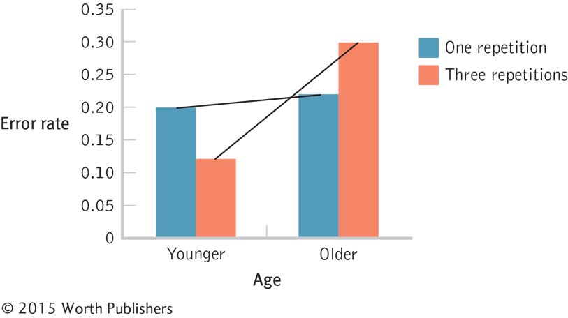
Interpreting the Interaction
The nonparallel lines demonstrate the interaction. The bars tell us that, on average, repetition decreases errors for younger people but increases them for older people. Because the direction reverses, this is a qualitative interaction.
Effect Size for Two-Way ANOVA
With a two-
MASTERING THE FORMULA
12-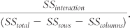
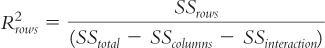
For the first main effect, the one in the rows of the table of cells, the formula is:
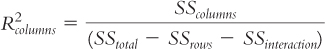
For the second main effect, the one in the columns of the table of cells, the formula is:
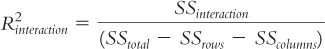
For the interaction, the formula is:
EXAMPLE 12.5
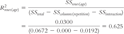
Let’s apply this to the ANOVA we just conducted. We use the statistics in the source table shown in Table 12-19 to calculate R2 for each main effect and the interaction. Here are the calculations for the main effect for age:
Here are the calculations for the main effect for repetitions:
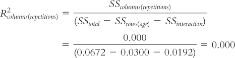
Here are the calculations for the interaction:
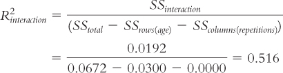
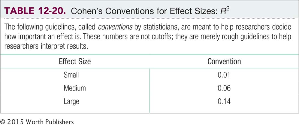
The conventions are the same as those presented in Chapter 11, shown again here in Table 12-20. From this table, we can see that the R2 of 0.63 for the main effect of age and 0.52 for the interaction are very large. The R2 of 0.00 for the main effect of repetitions indicates that there is no observable effect in this study.
CHECK YOUR LEARNING
| Reviewing the Concepts |
|
|||||||||||||
| Clarifying the Concepts | 12- |
What is the basic difference between the six steps of hypothesis testing for a two- |
||||||||||||
| 12- |
What are the four sources of variability in a two- |
|||||||||||||
| Calculating the Statistics | 12- |
Compute the three between- IV 1, level A; IV 2, level A: 2, 1, 1, 3 IV 1, level B; IV 2, level A: 5, 4, 3, 4 IV 1, level A; IV 2, level B: 2, 3, 3, 3 IV 1, level B; IV 2, level B: 3, 2, 2, 3 |
||||||||||||
| 12- |
Using the degrees of freedom you calculated in Check Your Learning 12- |
|||||||||||||
| Applying the Concepts | 12- |
Researchers studied the effect of e-
|
Solutions to these Check Your Learning questions can be found in Appendix D.