nolanessentials3e

8.2 Effect Size

As we learned when we looked at the research on gender differences in mathematical reasoning ability, “statistically significant” does not mean that the findings from a study represent a meaningful difference. “Statistically significant” only means that those findings are unlikely to occur if in fact the null hypothesis is true. Researcher Geoff Cumming, a vocal advocate for the use of the procedures taught in this chapter, points out that hypothesis testing “relies on strange backward logic and can’t give us direct information about what we want to know—the effect itself” (Cumming, 2014). Calculating an effect size moves us a little closer to the question we are most interested in: Is the pattern in a data set meaningful or important?

192

The Effect of Sample Size on Statistical Significance

Misinterpreting Statistical Significance Statistical significance that is achieved by merely collecting a large sample can make a research finding appear to be far more important than it really is, just as a curved mirror can exaggerate a person’s size.

Digital Vision, Ltd./Superstock

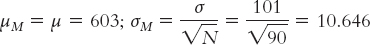
The almost completely overlapping curves in Figure 8-1 were “statistically significant” because the sample size was so big. Increasing sample size always increases the test statistic if all else stays the same. For example, psychology test scores on the Graduate Record Examination (GRE) had a mean of 603 and a standard deviation of 101 during the years 2005–2008 (http://www.ets.org). In a fictional study, Example 7.4 in Chapter 7, we reported that 90 graduating seniors had a mean of 622. Based on the sample size of 90, we reported the mean and standard error for the distribution of means as:

The test statistic calculated from these numbers was:

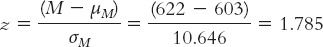
What would happen if we increased the sample size to 200? We’d have to recalculate the standard error to reflect the larger sample, and then recalculate the test statistic to reflect the smaller standard error.

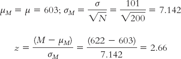
What if we increased the sample size to 1000?

What if we increased it to 100,000?

Notice that each time we increased the sample size, the standard error decreased and the test statistic increased. The original test statistic, 1.78, was not beyond the critical values of 1.96 and −1.96. However, the remaining test statistics (2.66, 5.95, and 59.56) were increasingly more extreme than the positive critical value. In their study of gender differences in mathematics performance, researchers studied 10,000 participants, a very large sample (Benbow & Stanley, 1980). It is not surprising, then, that a small difference would be a statistically significant difference.

193

MASTERING THE CONCEPT

8-2: As sample size increases, so does the test statistic (if all else stays the same). Because of this, a small difference might not be statistically significant with a small sample but might be statistically significant with a large sample.

Let’s consider, logically, why it makes sense that a large sample should allow us to reject the null hypothesis more readily than a small sample. If we randomly selected 5 people among all those who had taken the GRE and they had scores well above the national average, we might say, “It could be chance.” But if we randomly selected 1000 people with GRE scores well above the national average, it is very unlikely that we just happened to choose 1000 people with high scores.

But just because a real difference exists does not mean it is a large, or meaningful, difference. The difference we found with 5 people might be the same as the difference we found with 1000 people. As we demonstrated with multiple z tests with different sample sizes, we might fail to reject the null hypothesis with a small sample but then reject the null hypothesis for the same-size difference between means with a large sample.

Cohen (1990) used the small but statistically significant correlation between height and IQ to explain the difference between statistical significance and practical importance. The sample size was big: 14,000 children. Imagining that height and IQ were causally related, Cohen calculated that a person would have to grow by 3.5 feet to increase her IQ by 30 points (two standard deviations). Or, to increase her height by 4 inches, she would have to increase her IQ by 233 points! Height may have been statistically significantly related to IQ, but there was no practical real-world application. A larger sample size should influence the level of confidence that the story is true, but it should not increase our confidence that the story is important.

Language Alert! When you come across the term statistical significance, do not interpret this as an indication of practical importance.

Larger Samples Give Us More Confidence in Our Conclusions Stephen, a British student studying in the United States, is told that he won’t be able to find his favorite candy bar, Yorkie. He tests this hypothesis in 3 stores and finds no Yorkie bars. Another British student, Victoria, also warned by her friends, looks for her favorite, Curly Wurly. She tests her hypothesis in 25 U.S. stores and finds no Curly Wurly bars. Both conclude that their friends were right. Do you feel more confident that Stephen or Victoria really won’t be able to find their favorite candy bar?

What Effect Size Is

194

Effect size indicates the size of a difference and is unaffected by sample size.

Effect size can tell us whether a statistically significant difference might also be an important difference. Effect size indicates the size of a difference and is unaffected by sample size. Effect size tells us how much two populations do not overlap. Simply put, the less overlap, the bigger the effect size.

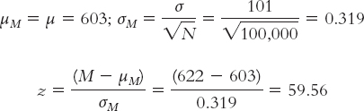
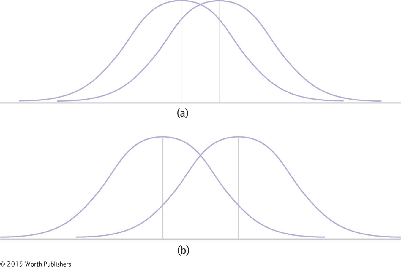
The amount of overlap between two distributions can be decreased in two ways. First, as shown in Figure 8-6, overlap decreases and effect size increases when means are further apart. Second, as shown in Figure 8-7, overlap decreases and effect size increases when variability within each distribution of scores is smaller.

Figure 8.6: FIGURE 8-6
Effect Size and Mean Differences
When two population means are farther apart, as in (b), the overlap of the distributions is less and the effect size is bigger.

Figure 8.7: FIGURE 8-7
Effect Size and Standard Deviation
When two population distributions decrease their spread, as in (b), the overlap of the distributions is less and the effect size is bigger.

When we discussed gender differences in mathematical reasoning ability, you may have noticed that we described the size of the findings as “small” (Hyde, 2005). Because effect size is a standardized measure based on scores rather than means, we can compare the effect sizes of different studies with one another, even when the studies have different sample sizes.

195

EXAMPLE 8.3

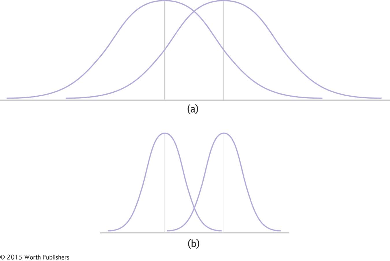
Figure 8-8 demonstrates why we use scores instead of means to calculate effect size. First, assume that each of these distributions is based on the same underlying population. Second, notice that all means represented by the vertical lines are identical. The differences are due only to the spread of the distributions. The small degree of overlap in the tall, skinny distributions of means in Figure 8-8a is the result of a large sample size. The greater degree of overlap in the somewhat wider distributions of means in Figure 8-8b is the result of a smaller sample size. By contrast, the distributions of scores in Figures 8-8c and 8-8d represent scores rather than means for these two studies. Because these flatter, wider distributions include actual scores, sample size is not an issue in making comparisons.

196

Figure 8.8: FIGURE 8-8
Making Fair Comparisons
The top two pairs of curves (a and b) depict two studies, study 1 and study 2. The first study (a) compared two samples with very large sample sizes, so each curve is very narrow. The second study (b) compared two samples with much smaller sample sizes, so each curve is wider. The first study has less overlap, but that doesn’t mean it has a bigger effect than study 2; we just can’t compare the effects. The bottom two pairs (c and d) depict the same two studies, but used standard deviation for the individual scores. Now they are comparable and we see that they have the same amount of overlap—the same effect sizes.

In this case, the amounts of real overlap in Figures 8-8c and 8-8d are identical. We can directly compare the amount of overlap and see that they have the same effect size.

Cohen’s d

105

Cohen’s d is a measure of effect size that assesses the difference between two means in terms of standard deviation, not standard error.

There are many different effect-size statistics, but they all neutralize the influence of sample size. When we conduct a z test, the effect-size statistic is typically Cohen’s d, developed by Jacob Cohen (Cohen, 1988). Cohen’s d is a measure of effect size that assesses the difference between two means in terms of standard deviation, not standard error. In other words, Cohen’s d allows us to measure the difference between means using standard deviations, much like a z statistic. We accomplish this by using standard deviation in the denominator (rather than using standard error).

EXAMPLE 8.4

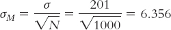
Let’s calculate Cohen’s d for the same data with which we constructed a confidence interval. We simply substitute standard deviation for standard error. When we calculated the test statistic for the 1000 customers at Starbucks with posted calories, we first calculated standard error:

MASTERING THE FORMULA

8-2: The formula for Cohen’s d for a z statistic is: Cohen’s d.

It is the same formula as for the z statistic, except we divide by the population standard deviation rather than by standard error.

We calculated the z statistic using the population mean of 247 and the sample mean of 232:

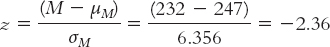
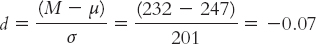
To calculate Cohen’s d, we simply use the formula for the z statistic, substituting σ for σ_M (and µ for µ_M, even though these means are always the same). So we use 201 instead of 6.356 in the denominator. Cohen’s d is based on the spread of the distribution of scores, rather than the distribution of means.

MASTERING THE CONCEPT

8-3: Because a statistically significant effect might not be an important one, we should calculate effect size in addition to conducting a hypothesis test. We can then report whether a statistically significant effect is small, medium, or large.

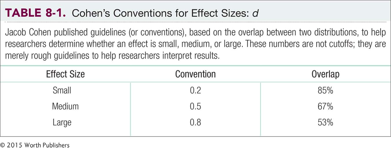
Now that we have the effect size, often written in shorthand as d = −0.07, we ask: What does it mean? First, we know that the two sample means are 0.07 standard deviation apart, which doesn’t sound like a big difference—and it isn’t. Cohen developed guidelines for what constitutes a small effect (0.2), a medium effect (0.5), and a large effect (0.8). Table 8-1 displays these guidelines, along with the amount of overlap between two curves that is indicated by an effect of that size. No sign is provided because it is the magnitude of an effect size that matters; an effect size of −0.5 is the same size as one of 0.5.

197

Based on these numbers, the effect size for the study of Starbucks customers (−0.07) is not even at the level of a small effect. As we pointed out in Chapter 7, however, the researchers hypothesized that even a small effect might spur eateries to provide more low-calorie choices. Sometimes a small effect can be meaningful.

Meta-Analysis

A meta-analysis is a study that involves the calculation of a mean effect size from the individual effect sizes of many studies.

Many researchers consider meta-analysis to be the most important recent advancement in social science research (e.g., Newton & Rudestam, 1999). A meta-analysis is a study that involves the calculation of a mean effect size from the individual effect sizes of many studies. Meta-analysis provides added statistical power by considering many studies simultaneously and helps to resolve debates fueled by contradictory research findings (Lam & Kennedy, 2005).

The logic of the meta-analysis process is surprisingly simple. There are just four steps:

Step 1: Select the topic of interest, and decide exactly how to proceed before beginning to track down studies.

Step 2: Locate every study that has been conducted and meets the criteria.

Step 3: Calculate an effect size, often Cohen’s d, for every study.

Step 4: Calculate statistics—ideally, summary statistics, a hypothesis test, a confidence interval, and a visual display of the effect sizes (Rosenthal, 1995).

In Step 4, researchers calculate a mean effect size for all studies, the central goal of a meta-analysis. They also apply all of the statistical insights we’ve learned: means, medians, standard deviations, confidence intervals and hypothesis testing, and graphs. The goal of hypothesis testing with meta-analysis is to reject the null hypothesis that the mean effect size is 0.

CHECK YOUR LEARNING

Reviewing the Concepts		As sample size increases, the test statistic becomes more extreme and it becomes easier to reject the null hypothesis. A statistically significant result is not necessarily one with practical importance. Effect sizes are calculated with respect to scores, rather than means, so they are not contingent on sample size. The size of an effect is based on the difference between two group means and the amount of variability within each group. Effect size for a z test is measured with Cohen’s d, which is calculated much like a z statistic, but using standard deviation instead of standard error. A meta-analysis is a study of studies that provides a more objective measure of an effect size than an individual study does.
198 Clarifying the Concepts	8-4	Distinguish statistical significance and practical importance.
	8-5	What is effect size?
Calculating the Statistics	8-6	Using IQ as a variable, where we know the mean is 100 and the standard deviation is 15, calculate Cohen’s d for an observed mean of 105.
Applying the Concepts	8-7	In Check Your Learning 8-3, you calculated a confidence interval based on CFC data. The population mean CFC score was 3.20, with a standard deviation of 0.70. The mean for the sample of 45 students who joined a career discussion group is 3.45. Calculate the appropriate effect size for this study. Citing Cohen’s conventions, explain what this effect size tells us. Based on the effect size, does this finding have any consequences or implications for anyone’s life?

Solutions to these Check Your Learning questions can be found in Appendix D.