14.2 Understanding Interactions in ANOVA
Back in the 1970s, media attention about NASA’s mission to Mars helped sell more Mars candy bars. Media attention primed the word Mars, which made Mars candy bars come to mind more easily. Priming, of course, would not increase sales for everybody—
In this section, we explore the concept of an interaction in a two-
356
Interactions and Public Policy

Hurricane Katrina demonstrates the importance of understanding interactions. First, the 2005 hurricane itself was an interaction among several weather variables. The devastating effects of the hurricane depended on particular levels of other variables, such as where it made landfall and the speed of its movement across the Gulf of Mexico.
Interactions were relevant for the people affected by Hurricane Katrina as well. For example, one would think that Hurricane Katrina would have been universally bad for the health of all those displaced people—
Some women gave birth in the squalor of the public shelter in New Orleans’ Superdome or in alleys while waiting for rescuers. When it comes to pregnant women, the first priority of disaster relief agencies is to provide obstetric and neonatal care. Massive relief efforts sometimes mean that access to care for pregnant women is actually improved in the aftermath of a disaster. Of course, the quality of health care certainly doesn’t improve for everybody, which means that an interaction is involved. So the quality of health care improved for pregnant women in the aftermath of the disaster, whereas it became worse for almost everyone else. In the language of two-
Interpreting Interactions
The two-
A quantitative interaction is an interaction in which the effect of one independent variable is strengthened or weakened at one or more levels of the other independent variable, but the direction of the initial effect does not change.
Quantitative Interactions Two terms often used to describe interactions are quantitative and qualitative (e.g., Newton & Rudestam, 1999). A quantitative interaction is an interaction in which the effect of one independent variable is strengthened or weakened at one or more levels of the other independent variable, but the direction of the initial effect does not change. The researcher ski bums, Jonathan Zinman and Eric Zitzewitz, found a quantitative interaction when they discovered that resort snowfall reports were always exaggerated compared to weather reports, and especially on the weekends. More specifically, the effect of one independent variable is modified in the presence of another independent variable.
357
A qualitative interaction is a particular type of quantitative interaction of two (or more) independent variables in which one independent variable reverses its effect depending on the level of the other independent variable.
A qualitative interaction is a particular type of quantitative interaction of two (or more) independent variables in which one independent variable reverses its effect depending on the level of the other independent variable. In a qualitative interaction, the effect of one variable doesn’t just become stronger or weaker; it actually reverses direction in the presence of another variable. Let’s first examine the quantitative interaction.
MASTERING THE CONCEPT
14.2: Researchers often describe interactions with one of two terms—
EXAMPLE 14.2
The grapefruit juice example is a helpful illustration of a quantitative interaction. Lipitor and Zocor lead to elevations of some liver enzymes in combination with water, but the absorption levels are even higher with grapefruit juice. This effect is not seen with a placebo, which has an equal effect regardless of beverage. Let’s invent some numbers to demonstrate this. The numbers in the cells in Table 14-4 don’t represent actual absorption levels; rather, they are numbers that are easy for us to work with in our understanding of interactions. For this exercise, we will consider every difference between numbers to be statistically significant. (Of course, if we really conducted this study, we would conduct the two-
| Lipitor | Zocor | Placebo | ||
|---|---|---|---|---|
| Grapefruit juice | 60 | 60 | 3 | 41 |
| Water | 30 | 30 | 3 | 21 |
| 45 | 45 | 3 |
First, we consider main effects; then we consider the overall pattern that constitutes the interaction. If there is a significant interaction, we ignore any significant main effects. The significant interaction supersedes any significant main effects.
A marginal mean is the mean of a row or a column in a table that shows the cells of a study with a two-
Table 14-4 includes mean absorption levels for the six cells of the study. It also includes numbers in the margins of the table, to the right of and below the cells; these numbers are also means, but are for every participant in a given row or in a given column. Each of these is called a marginal mean, the mean of a row or a column in a table that shows the cells of a study with a two-
The easiest way to understand the main effects is to make a smaller table for each, with only the appropriate marginal means. Separate tables let us focus on one main effect at a time without being distracted by the means in the cells. For the main effect of beverage, we construct a table with two cells, as shown in Table 14-5. The table makes it easy to see that the absorption level was higher, on average, for grapefruit juice than for water.
| Grapefruit juice | 41 |
| Water | 21 |
358
Let’s now consider the second main effect, that for medication. As before, we construct a table (such as Table 14-6) that shows only the means for medication, as if beverage were not included in the study. We kept the means for beverage in rows and for medication in columns, just as they were in the original table. You may, however, arrange them either way, using whichever order makes sense to you. Table 14-6 shows that the absorption levels for Lipitor and Zocor were higher, on average, than for placebo, which led to almost no absorption. Both results would need to be verified with a hypothesis test, but we seem to have two main effects: (1) a main effect of beverage (grapefruit juice leads to higher absorption, on average, than water does), and (2) a main effect of medication (Lipitor and Zocor lead to higher absorption, on average, than placebo does).
| Lipitor | Zocor | Placebo |
|---|---|---|
| 45 | 45 | 3 |
But that’s not the whole story. Grapefruit juice, for example, does not lead to higher absorption, on average, among placebo users. Here’s where the interaction comes in. Now we ignore the marginal means and get back to the means in the cells themselves, seen again in Table 14-7. Here we can see the overall pattern by framing it in two different ways. We can start by considering beverage. Does grapefruit juice boost mean absorption levels as compared to water? It depends. It depends on the level of the other independent variable, medication; specifically, it depends on whether the patient is taking one of the two medications or a placebo. We can also frame the question by starting with medication. Do Lipitor and Zocor boost mean absorption levels as compared to a placebo? It depends. They do anyway, even just in conjunction with water, but they do so to a far greater degree in conjunction with grapefruit juice. This is a quantitative interaction because the strength of the effect varies under certain conditions, but the direction does not.
| Lipitor | Zocor | Placebo | |
|---|---|---|---|
| Grapefruit juice | 60 | 60 | 3 |
| Water | 30 | 30 | 3 |
People sometimes perceive an interaction where there is none. If Lipitor, Zocor, and a placebo all had higher mean absorption rates in conjunction with grapefruit juice (versus water), there would be no interaction. Lipitor and Zocor would always lead to a particular increase in average absorption levels versus a placebo—
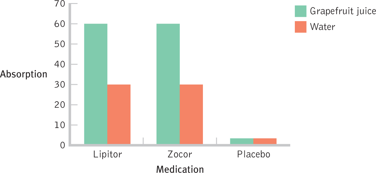
Figure 14-
359
The bar graph helps us to see the overall pattern, but one more step is necessary: to connect each set of bars with a line. We have two choices that match the two ways we framed the interaction in words above: (1) As in Figure 14-3, we could connect the bars for the first independent variable, medication. We would connect the three medications for the grapefruit condition, and then we would connect the three medications for the water condition. (2) Alternatively, as in Figure 14-4, we could connect the bars for the two beverages. We would connect the two beverages for Lipitor, for Zocor, and for placebo.
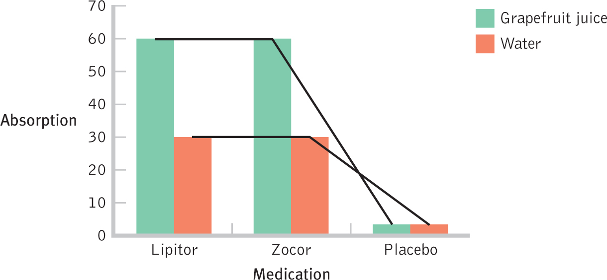
Figure 14-
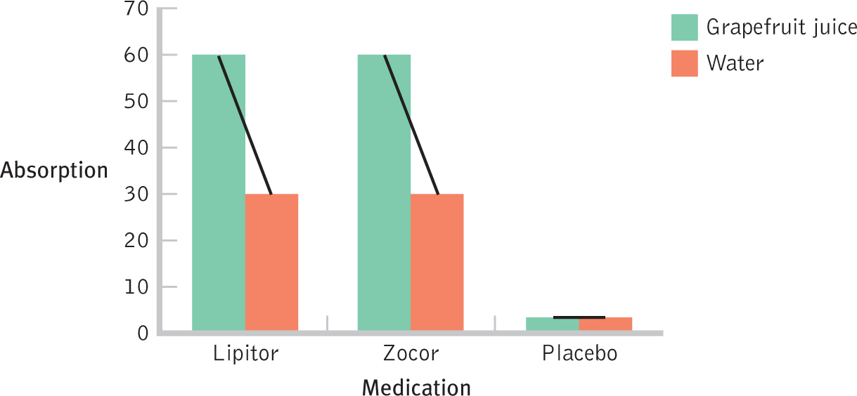
Figure 14-
360
In Figure 14-4, notice that the lines do not intersect, but they’re not all parallel to one another either. If the lines were extended far enough, eventually the lines connecting the two bars for each medication would intersect the line connecting the bar for placebo. Perfectly parallel lines indicate the likely absence of an interaction, but we almost never see perfectly parallel lines emerging from real-
Some social scientists refer to an interaction as a significant difference in differences. In the context of the grapefruit juice study, the mean difference between grapefruit juice and water is larger when participants are taking one of the medications than when they are taking the placebo. In fact, for those taking the placebo, there is no mean difference between grapefruit juice and water. This is an example of a significant difference between differences. This interaction is represented graphically whenever the lines connecting the bars are significantly different from parallel.
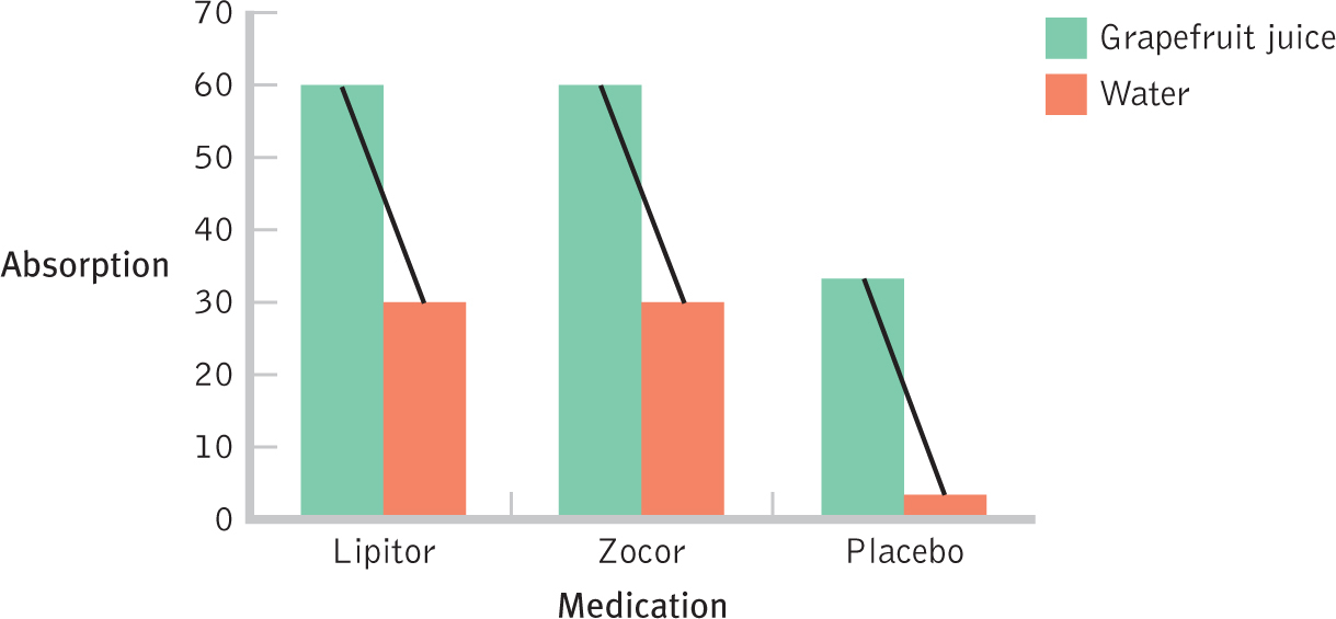
Figure 14-
However, if grapefruit juice also led to an increase in mean absorption levels among those taking the placebo, the graph would look like the one in Figure 14-5. In this case, the mean absorption levels of Lipitor and Zocor do increase with grapefruit juice, but so does the mean absorption level of the placebo, and there is likely no interaction. Grapefruit juice has the same effect, regardless of the level of the other independent variable of medication. When in doubt about whether there is an interaction or just two main effects that add up to a greater effect, draw a graph and connect the bars with lines. However, don’t just draw lines and skip the step of creating the bar graph. Zacks and Tversky (1997) reported that some people view lines as indicating a continuous variable, with a participant in one of their experiments viewing a line graph and stating: “The more male a person is, the taller he/she is” (p. 148). A bar graph would likely have led that participant to perceive, accurately, that men are, on average, taller than women.
Qualitative Interactions Let’s recall the definition of a qualitative interaction: a particular type of quantitative interaction in which the effect of one independent variable reverses its effect depending on the level of the other independent variable.
361
EXAMPLE 14.3
Do you think that, on average, people make better decisions when they consciously focus on the decision? Or do they make better decisions when the decision-
In one study, participants were asked to choose one of four cars. One car was objectively the best of the four, and one was objectively the worst. Some participants made a less complex decision; they were told 4 characteristics of each car. Some participants made a more complex decision; they were told 14 characteristics of each car. After learning about the cars, half the participants in each group were randomly assigned to think consciously about the cars for 4 minutes before making a decision. Half were randomly assigned to distract themselves for 4 minutes by solving anagrams before making a decision. The research design, with two independent variables, is shown in Table 14-8. The first independent variable is complexity, with two levels: less complex (4 attributes) and more complex (14 attributes). The second independent variable is type of decision making, with two levels: conscious thought and unconscious thought (distraction).
| Conscious Thought | Unconscious Thought (Distraction) | |
|---|---|---|
| Less complex (4 attributes of each car) | Less complex; conscious | Less complex; unconscious |
| More complex (14 attributes of each car) | More complex; conscious | More complex; unconscious |
The researchers calculated a score for each participant that reflected his or her ability to differentiate between the objectively best and objectively worst cars in the group. This score represents the dependent variable, and higher numbers indicate a better ability to differentiate between the best and worst cars. Let’s look at Table 14-9, which presents cell means and marginal means for this experiment. Note that the means are approximate and that the marginal means are created by assuming the same number of participants in each cell. As we consider these findings, we will assume that all differences are statistically significant. (In a real research situation, we would conduct an ANOVA to determine statistical significance.)

| Conscious Thought | Unconscious Thought (Distraction) | ||
|---|---|---|---|
| Less complex | 5.5 | 2.3 | 3.9 |
| More complex | 0.6 | 5.0 | 2.8 |
| 3.05 | 3.65 |
362
Because there was an overall pattern—
| Less complex | 3.9 |
| More complex | 2.8 |
| Conscious | Unconscious |
|---|---|
| 3.05 | 3.65 |
However, if there is also a significant interaction, these main effects don’t tell the whole story. The overall pattern of cell means renders this information misleading, even inaccurate, under certain conditions. The interaction demonstrates that the effect of the decision-
A bar graph, shown in Figure 14-6, makes the pattern of the data far clearer. We can actually see the qualitative interaction.
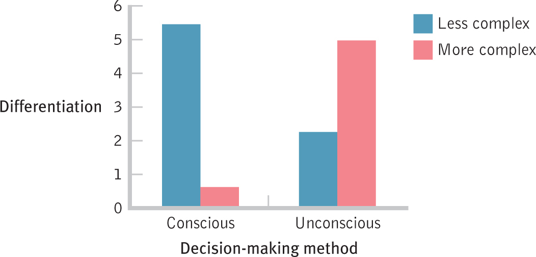
Figure 14-
As we do with a quantitative interaction, we add lines to determine whether they are parallel (no matter how long the lines are) or intersect (or would do so if extended far enough), as in Figure 14-7. Here we see that the lines intersect without even having to extend them beyond the graph. This is likely an interaction. Type of decision making has an effect on differentiation between best and worst cars, but it depends on the complexity of the decision. Those making a less complex decision tend to make better choices if they use conscious thought. Those making a more complex decision tend to make better choices if they use unconscious thought. We would, as usual, verify this finding by conducting a hypothesis test before rejecting the null hypothesis that there is no interaction.
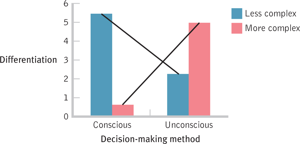
Figure 14-
363
The qualitative interaction of decision-
So what do these findings mean for us as we approach the decisions we face every day? Which sunblock should we buy to best protect against UV rays? Should we go to graduate school or get a job following graduation? Should we consciously consider characteristics of sunblocks but “sleep on” graduate school–
CHECK YOUR LEARNING
Reviewing the Concepts
- A two-
way ANOVA is represented by a grid in which cells represent each unique combination of independent variables. Means are calculated for cells, called cell means. Means are also computed for each level of an independent variable, by itself, regardless of the levels of the other independent variable. These means, found in the margins of the grid, are called marginal means. - When there is a statistically significant interaction, the main effects are considered to be modified by an interaction. As a result, we focus only on the overall pattern of cell means that reveals the interaction.
- Two categories of interactions describe the overall pattern of cell means—
quantitative and qualitative interactions. - The most common interaction is a quantitative interaction, in which the effect of the first independent variable depends on the levels of the second independent variable, but the differences at each level vary only in the strength of the effect.
- Qualitative interactions are those in which the effect of the first independent variable depends on the levels of the second independent variable, but the direction of the effect actually reverses.
- There are three ways to identify a statistically significant interaction: (1) visually, whenever the lines connecting the means of each group are significantly different from parallel; (2) conceptually, when you need to use the idea of “it depends” to tell the data’s story; and (3) statistically, when the p value associated with an interaction in a source table is < 0.05, as with other hypothesis tests. This last method, the statistical analysis, is the only objective way to assess the interaction.
Clarifying the Concepts
- 14-
5 What is the difference between a quantitative interaction and a qualitative interaction? - 14-
6 Why are main effects ignored when there is an interaction? (We often say they are trumped by an interaction.)
Calculating the Statistics
- 14-
7 Data are presented here for two hypothetical independent variables (IVs) and their combinations.
IV 1, level A; IV 2, level A: 2, 1, 1, 3
IV 1, level B; IV 2, level A: 5, 4, 3, 4
IV 1, level A; IV 2, level B: 2, 3, 3, 3
IV 1, level B; IV 2, level B: 3, 2, 2, 3- Figure out how many cells are in this study’s table, and draw a grid to represent them.
- Calculate cell means and write them in the cells of the grid.
- Calculate marginal means and write them in the margins of the grid.
- Draw a bar graph of these data.
Applying the Concepts
- 14-
8 For each of the following situations involving a real-life interaction, (i) state the independent variables, (ii) state the likely dependent variable, (iii) construct a table showing the cells, and (iv) explain whether the interaction is qualitative or quantitative. - Caroline and Mira are both really smart and do equally well in their psychology class, but something happens to Caroline when she goes to their philosophy class. She just can’t keep up, whereas Mira does even better.
- Our college baseball team has had a great few years. The team plays especially well at home versus away when playing teams in its own conference. However, it plays especially well at away games (versus home games) when playing teams from another conference.
- Caffeinated drinks get me wired and make it somewhat difficult for me to sleep. So does working out in the evenings. When I do both, I’m so wired that I might as well stay up all night.
Solutions to these Check Your Learning questions can be found in Appendix D.