10.1 Inference about the Regression Model
 This page includes Video Technology Manuals
 This page includes Statistical Videos
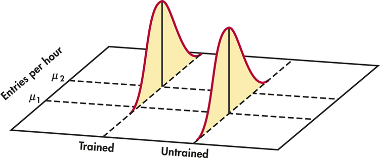
Simple linear regression studies the relationship between a response variable y and an explanatory variable x. We expect that different values of x are associated with different mean responses for y. We encountered a similar but simpler situation in Chapter 7 when we discussed methods for comparing two population means. Figure 10.1 illustrates a statistical model for comparing the items per hour entered by two groups of financial clerks using new data entry software. Group 2 received some training in the software while Group 1 did not. Entries per hour is the response variable. The treatment (training or not) is the explanatory variable. The model has two important parts:
- The mean entries per hour may be different in the two populations. These means are μ1 and μ2 in Figure 10.1.
- Individual entries per hour vary within each population according to a Normal distribution. The two Normal curves in Figure 10.1 describe these responses. These Normal distributions have the same spread, indicating that the population standard deviations are assumed to be equal.
Statistical model for simple linear regression
Now imagine giving different lengths x of training to different groups of subjects. We can think of these groups as belonging to subpopulations, one for each possible value of x. Each subpopulation consists of all individuals in the population having the same value of x. If we gave x=15 hours of training to some subjects, x=30 hours of training to some others, and x=60 hours of training to some others, these three groups of subjects would be considered samples from the corresponding three subpopulations.
subpopulation
The statistical model for simple linear regression also assumes that, for each value of x, the response variable y is Normally distributed with a mean that depends on x. We use μy to represent these means. In general, the means μy can change as x changes according to any sort of pattern. In simple linear regression, we assume that the means all lie on a line when plotted against x. To summarize, this model also has two important parts:
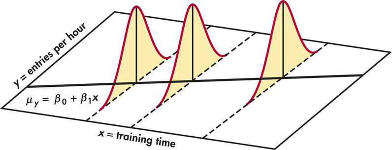
- The mean entries per hour μy changes as the number of training hours x changes. The means all lie on a straight line. That is, μy=β0+β1x.
- Individual entries per hour y for subjects with the same amount of training x vary according to a Normal distribution. This variation, measured by the standard deviation σ, is the same for all values of x.
This statistical model is pictured in Figure 10.2. The line describes how the mean response μy changes with x. This is the population regression line. The three Normal curves show how the response y will vary for three different values of the explanatory variable x. Each curve is centered at its mean response μy. All three curves have the same spread, measured by their common standard deviation σ.
population regression line
From data analysis to inference

The data for a regression problem are the observed values of x and y. The model takes each x to be a fixed known quantity, like the hours of training a worker has received.1 The response y for a given x is a Normal random variable. The model describes the mean and standard deviation of this random variable. This model is not appropriate if there is error in measuring x and it is large relative to the spread of the x’s. In these situations, more advanced inference methods are needed.
We use Case 10.1 to explain the fundamentals of simple linear regression. Because regression calculations in practice are always done by software, we rely on computer output for the arithmetic. Later in the chapter, we show formulas for doing the calculations. These formulas are useful in understanding analysis of variance (see Section 10.3) and multiple regression (see Chapter 11).


Numerous studies have shown that better-educated employees have higher incomes. Is this also true for entrepreneurs? Do more years of formal education translate into higher incomes? And if so, is the return for an additional year of education the same for entrepreneurs and employees? One study explored these questions using the National Longitudinal Survey of Youth (NLSY), which followed a large group of individuals aged 14 to 22 for roughly 10 years.2 They looked at both employees and entrepreneurs, but we just focus on entrepreneurs here.
entre
The researchers defined entrepreneurs to be those who were self-employed or who were the owner/director of an incorporated business. For each of these individuals, they recorded the education level and income. The education level (EDUC) was defined as the years of completed schooling prior to starting the business. The income level was the average annual total earnings (INC) since starting the business.
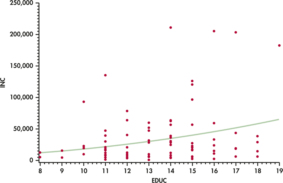
We consider a random sample of 100 entrepreneurs. Figure 10.3 is a scatterplot of the data with a fitted smoothed curve. The explanatory variable x is the entrepreneur’s education level. The response variable y is the income level.
Let’s briefly review some of the ideas from Chapter 2 regarding least-squares regression. We start with a plot of the data, as in Figure 10.3, to verify that the relationship is approximately linear with no outliers. Always start with a graphical display of the data. There is no point in fitting a linear model if the relationship does not, at least approximately, appear linear. In this case, the distribution of income is skewed to the right (at each education level, there are many small incomes and just a few large incomes). Although the smoothed curve is roughly linear, the curve is being pulled toward the very large incomes, suggesting these observations could be influential.

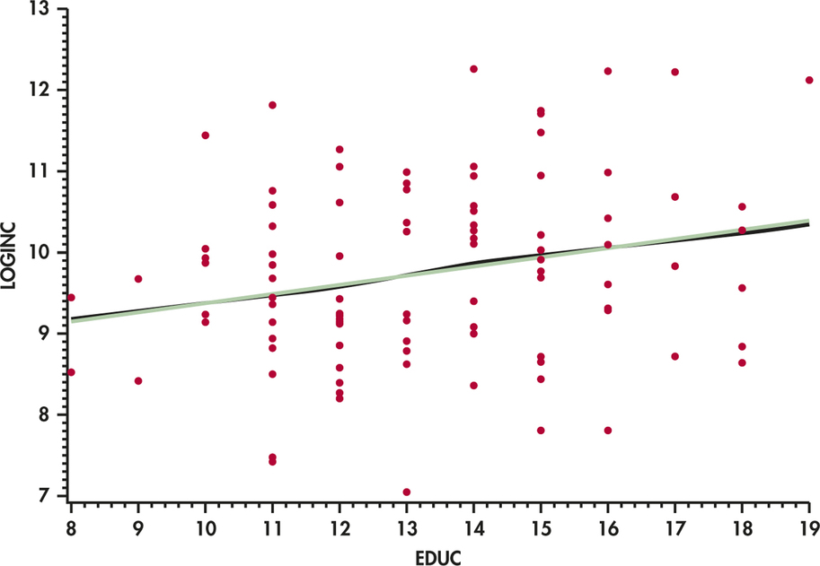
A common remedy for a strongly skewed variable such as income is to consider transforming the variable prior to fitting a model. Here, the researchers considered the natural logarithm of income (LOGINC). Figure 10.4 is a scatterplot of these transformed data with a fitted smoothed curve in black and the least-squares regression line in green. The smoothed curve is almost linear, and the observations in the y direction are more equally dispersed above and below this curve than the curve in Figure 10.3. Also, those four very large incomes no longer appear to be influential. Given these results, we continue our discussion of least-squares regression using the transformed y data.
EXAMPLE 10.1 Prediction of Log Income from Education Level
entre
CASE 10.1 The green line in Figure 10.4 is the least-squares regression line for predicting log income from years of formal schooling. The equation of this line is
predicted LOGINC=8.2546+0.1126×EDUC
We can use the least-squares regression equation to find the predicted log income corresponding to a given value of EDUC. The difference between the observed and predicted value is the residual. For example, Entrepreneur 4 has 15 years of formal schooling and a log income of 10.2274. We predict that this person will have a log income of
8.2546+(0.1126)(15)=9.9436
so the residual is
y−ˆy=10.2274−9.9436=0.2838
Recall that the least-squares line is the line that minimizes the sum of the squares of the residuals. The least-squares regression line also always passes through the point (ˉx, ˉy). These are helpful facts to remember when considering the fit of this line to a data set.
In Section 2.2 (pages 74–77), we discussed the correlation as a measure of association between two quantitative variables. In Section 2.3, we learned to interpret the square of the correlation as the fraction of the variation in y that is explained by x in a simple linear regression.
EXAMPLE 10.2 Correlation between Log Income and Education Level
CASE 10.1 For Case 10.1, the correlation between LOGINC and EDUC is r=0.2394. Because the squared correlation r2=0.0573, the change in log income along the regression line as years of education increases explains only 5.7% of the variation. The remaining 94.3% is due to other differences among these entrepreneurs. The entrepreneurs in this sample live in different parts of the United States; some are single and others are married; and some may have had a difficult upbringing. All these factors could be associated with log income and thus add to the variability if not included in the model.
Apply Your Knowledge
Question 10.1
10.1 Predict the log income.
In Case 10.1, Entrepreneur 3 has an EDUC of 14 years and a log income of 10.9475. Using the least-squares regression equation in Example 10.1, find the predicted log income and the residual for this individual.
10.1
ˆy=9.831. Residual=1.1165.
Question 10.2
10.2 Understanding a linear regression model.
Consider a linear regression model with μy=26.35+3.4x and standard deviation σ=4.1.
- What is the slope of the population regression line?
- Explain clearly what this slope says about the change in the mean of y for a unit change in x.
- What is the subpopulation mean when x=12?
- Between what two values would approximately 95% of the observed responses y fall when x=12?
Having reviewed the basics of least-squares regression, we are now ready to proceed with a discussion of inference for regression. Here’s what is new in this chapter:
- We regard the 100 entrepreneurs for whom we have data as a simple random sample (SRS) from the population of all entrepreneurs in the United States.
- We use the regression line calculated from this sample as a basis for inference about the population. For example, for a given level of education, we want not just a prediction but a prediction with a margin of error and a level of confidence for the log income of any entrepreneur in the United States.
Our statistical model assumes that the responses y are Normally distributed with a mean μy that depends upon x in a linear way. Specifically, the population regression line
μy=β0+β1x
describes the relationship between the mean log income μy and the number of years of formal education x in the population. The slope β1 is the mean increase in log income for each additional year of education. The intercept β0 is the mean log income when an entrepreneur has x=0 years of formal education. This parameter, by itself, is not meaningful in this example because x=0 years of education would be extremely rare.
Because the means μy lie on the line μy=β0+β1x, they are all determined by β0 and β1. Thus, once we have estimates of β0 and β1, the linear relationship determines the estimates of μy for all values of x. Linear regression allows us to do inference not only for subpopulations for which we have data, but also for those corresponding to x’s not present in the data. These x-values can be both within and outside the range of observed x’s. However, extreme caution must be taken when performing inference for an x-value outside the range of the observed x’s because there is no assurance that the same linear relationship between μy and x holds.
We cannot observe the population regression line because the observed responses y vary about their means. In Figure 10.4 we see the least-squares regression line that describes the overall pattern of the data, along with the scatter of individual points about this line. The statistical model for linear regression makes the same distinction. This was displayed in Figure 10.2 with the line and three Normal curves. The population regression line describes the on-the-average relationship and the Normal curves describe the variability in y for each value of x.
Think of the model in the form
DATA=FIT+RESIDUAL
The FIT part of the model consists of the subpopulation means, given by the expression β0+β1x. The RESIDUAL part represents deviations of the data from the line of population means. The model assumes that these deviations are Normally distributed with standard deviation σ. We use ∈ (the lowercase Greek letter epsilon) to stand for the RESIDUAL part of the statistical model. A response y is the sum of its mean and a chance deviation ∈ from the mean. The deviations ∈ represent “noise,” variation in y due to other causes that prevent the observed (x, y)-values from forming a perfectly straight line on the scatterplot.
Simple Linear Regression Model
Given n observations of the explanatory variable x and the response variable y,
(x1, y1),(x2, y2),…,(xn, yn)
The statistical model for simple linear regression states that the observed response yi when the explanatory variable takes the value xi is
yi=β0+β1xi+∈i
Here, μy=β0+β1xi is the mean response when x=xi. The deviations ∈i are independent and Normally distributed with mean 0 and standard deviation σ.
The parameters of the model are β0, β1, and σ.
The simple linear regression model can be justified in a wide variety of circumstances. Sometimes, we observe the values of two variables, and we formulate a model with one of these as the response variable and the other as the explanatory variable. This was the setting for Case 10.1, where the response variable was log income and the explanatory variable was the number of years of formal education. In other settings, the values of the explanatory variable are chosen by the persons designing the study. The scenario illustrated by Figure 10.2 is an example of this setting. Here, the explanatory variable is training time, which is set at a few carefully selected values. The response variable is the number of entries per hour.
For the simple linear regression model to be valid, one essential assumption is that the relationship between the means of the response variable for the different values of the explanatory variable is approximately linear. This is the FIT part of the model. Another essential assumption concerns the RESIDUAL part of the model. The assumption states that the residuals are an SRS from a Normal distribution with mean zero and standard deviation σ. If the data are collected through some sort of random sampling, this assumption is often easy to justify. This is the case in our two scenarios, in which both variables are observed in a random sample from a population or the response variable is measured at predetermined values of the explanatory variable.
In many other settings, particularly in business applications, we analyze all of the data available and there is no random sampling. Here, we often justify the use of inference for simple linear regression by viewing the data as coming from some sort of process. The line gives a good description of the relationship, the fit, and we model the deviations from the fit, the residuals, as coming from a Normal distribution.
EXAMPLE 10.3 Retail Sales and Floor Space
It is customary in retail operations to assess the performance of stores partly in terms of their annual sales relative to their floor area (square feet). We might expect sales to increase linearly as stores get larger, with, of course, individual variation among stores of the same size. The regression model for a population of stores says that
sales=β0+β1×area+∈
The slope β1 is, as usual, a rate of change: it is the expected increase in annual sales associated with each additional square foot of floor space. The intercept β0 is needed to describe the line but has no statistical importance because no stores have area close to zero. Floor space does not completely determine sales. The ∈ term in the model accounts for differences among individual stores with the same floor space. A store’s location, for example, could be important but is not included in the FIT part of the model. In Chapter 11, we consider moving variables like this out of the RESIDUAL part of the model by allowing more than one explanatory variable in the FIT part.
Apply Your Knowledge
Question 10.3
10.3 U.S. versus overseas stock returns.
Returns on common stocks in the United States and overseas appear to be growing more closely correlated as economies become more interdependent. Suppose that the following population regression line connects the total annual returns (in percent) on two indexes of stock prices:
mean overseas return=−0.1+0.15×U.S. return
- What is β0 in this line? What does this number say about overseas returns when the U.S. market is flat (0% return)?
- What is β1 in this line? What does this number say about the relationship between U.S. and overseas returns?
- We know that overseas returns will vary in years that have the same return on U.S. common stocks. Write the regression model based on the population regression line given above. What part of this model allows overseas returns to vary when U.S. returns remain the same?
10.3
(a) −0.1. When the U.S. market is flat, the overseas returns will be −0.1. (b) 0.15. For each unit increase in U.S. return, the mean overseas return will increase by 0.15. (c) MEAN OVERSEAS RETURN=β0+β1×U.S. RETURN+ε. The ε allows overseas returns to vary when U.S. returns remain the same.
Question 10.4
10.4 Fixed and variable costs.
In some mass production settings, there is a linear relationship between the number x of units of a product in a production run and the total cost y of making these x units.
- Write a population regression model to describe this relationship.
- The fixed cost is the component of total cost that does not change as x increases. Which parameter in your model is the fixed cost?
- Which parameter in your model shows how total cost changes as more units are produced? Do you expect this number to be greater than 0 or less than 0? Explain your answer.
- Actual data from several production runs will not fall directly on a straight line. What term in your model allows variation among runs of the same size x?
Estimating the regression parameters
The method of least squares presented in Chapter 2 fits the least-squares line to summarize a relationship between the observed values of an explanatory variable and a response variable. Now we want to use this line as a basis for inference about a population from which our observations are a sample. We can do this only when the statistical model for regression is reasonable. In that setting, the slope b1 and intercept b0 of the least-squares line
ˆy=b0+b1x
estimate the slope β1 and the intercept β0 of the population regression line.
Recalling the formulas from Chapter 2, the slope of the least-squares line is
b1=rsysx
and the intercept is
b0=ˉy−b1ˉx
Here, r is the correlation between the observed values of y and x, sy is the standard deviation of the sample of y’s, and sx is the standard deviation of the sample of x’s. Notice that if the estimated slope is 0, so is the correlation, and vice versa. We discuss this relationship more later in this chapter.
The remaining parameter to be estimated is σ, which measures the variation of y about the population regression line. More precisely, σ is the standard deviation of the Normal distribution of the deviations ∈i in the regression model. However, we don’t observe these ∈i, so how can we estimate σ?
Recall that the vertical deviations of the points in a scatterplot from the fitted regression line are the residuals. We use ei for the residual of the ith observation:
ei=observed response−predicted response=yi−ˆyi=yi−b0−b1xi
The residuals ei are the observable quantities that correspond to the unobservable model deviations ∈i. The ei sum to 0, and the ∈i come from a population with mean 0. Because we do not observe the ∈i, we use the residuals to estimate σ and check the model assumptions of the ∈i.
To estimate σ, we work first with the variance and take the square root to obtain the standard deviation. For simple linear regression the estimate of σ2 is the average squared residual
s2=1n−2∑e2i=1n−2∑(yi−ˆyi)2
We average by dividing the sum by n−2 in order to make s2 an unbiased estimator of σ2. The sample variance of n observations use the divisor n−1 for the same reason. The residuals ei are not n separate quantities. When any n−2 residuals are known, we can find the other two. The quantity n−2 is the degrees of freedom of s2. The estimate of the model standard deviation σ is given by
s=√s2
model standard deviation σ
We call s the regression standard error.
Estimating the Regression Parameters
In the simple linear regression setting, we use the slope b1 and intercept b0 of the least-squares regression line to estimate the slope β1 and intercept β0 of the population regression line.
The standard deviation σ in the model is estimated by the regression standard error
s=√1n−2∑(yi−ˆyi)2
In practice, we use software to calculate b1, b0, and s from data on x and y. Here are the results for the income example of Case 10.1.
EXAMPLE 10.4 Log Income and Years of Education
entre
CASE 10.1 Figure 10.5 displays Excel output for the regression of log income (LOGINC) on years of education (EDUC) for our sample of 100 entrepreneurs in the United States. In this output, we find the correlation r=0.2394 and the squared correlation that we used in Example 10.2, along with the intercept and slope of the least-squares line. The regression standard error s is labeled simply “Standard Error.”
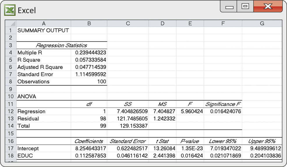
The three parameter estimates are
b0=8.254643317b1=0.112587853s=1.114599592
After rounding, the fitted regression line is
ˆy=8.2546+0.1126x
As usual, we ignore the parts of the output that we do not yet need. We will return to the output for additional information later.
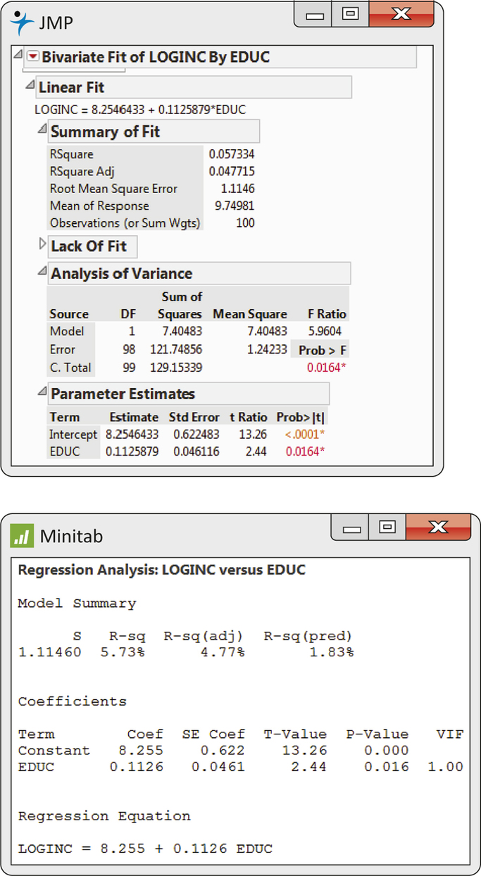
Figure 10.6 shows the regression output from two other software packages. Although the formats differ, you should be able to find the results you need. Once you know what to look for, you can understand statistical output from almost any software.
Apply Your Knowledge
Question 10.5
10.5 Research and development spending.
The National Science Foundation collects data on the research and development spending by universities and colleges in the United States.3 Here are the data for the years 2008–2011:
| Year | 2008 | 2009 | 2010 | 2011 |
|---|---|---|---|---|
| Spending (billions of dollars) | 51.9 | 54.9 | 58.4 | 62.0 |
- Make a scatterplot that shows the increase in research and development spending over time. Does the pattern suggest that the spending is increasing linearly over time?
- Find the equation of the least-squares regression line for predicting spending from year. Add this line to your scatterplot.
- For each of the four years, find the residual. Use these residuals to calculate the standard error s. (Do these calculations with a calculator.)
- Write the regression model for this setting. What are your estimates of the unknown parameters in this model?
- Use your least-squares equation to predict research and development spending for the year 2013. The actual spending for that year was $63.4 billion. Add this point to your plot, and comment on why your equation performed so poorly.
(Comment: These are time series data. Simple regression is often a good fit to time series data over a limited span of time. See Chapter 13 for methods designed specifically for use with time series.)
10.5
(a) The spending is increasing linearly over time. (b) ˆy=−6735.3+3.38x.
(c) 0.17, −0.21, −0.09, 0.13. s=0.22136.
(d) SPENDING=β0+β1×YEAR+ε. The estimate for β0 is −6735.5, the estimate for β1 is 3.38, and the estimate for ε is 0. (e) 68.63.
Conditions for regression inference
You can fit a least-squares line to any set of explanatory-response data when both variables are quantitative. The simple linear regression model, which is the basis for inference, imposes several conditions on this fit. We should always verify these conditions before proceeding to inference. There is no point in trying to do statistical inference if the data do not, at least approximately, meet the conditions that are the foundation for the inference.
The conditions concern the population, but we can observe only our sample. Thus, in doing inference, we act as if the sample is an SRS from the population. For the study described in Case 10.1, the researchers used a national survey. Participants were chosen to be a representative sample of the United States, so we can treat this sample as an SRS. The potential for bias should always be considered, especially when obtaining volunteers.
The next condition is that there is a linear relationship in the population, described by the population regression line. We can’t observe the population line, so we check this condition by asking if the sample data show a roughly linear pattern in a scatterplot. We also check for any outliers or influential observations that could affect the least-squares fit. The model also says that the standard deviation of the responses about the population line is the same for all values of the explanatory variable. In practice, the spread of observations above and below the least-squares line should be roughly the same as x varies.
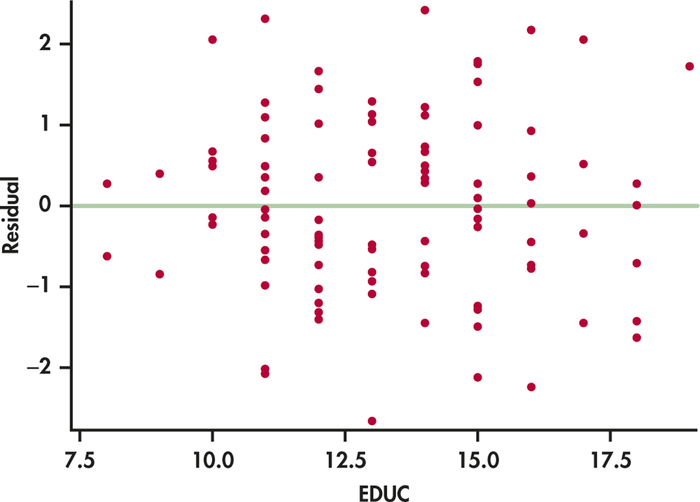
Plotting the residuals against the explanatory variable or against the predicted (or fitted) values is a helpful and frequently used visual aid to check these conditions. This is better than the scatterplot because a residual plot magnifies patterns. The residual plot in Figure 10.7 for the data of Case 10.1 looks satisfactory. There is no curved pattern or data points that seem out of the ordinary, and the data appear equally dispersed above and below zero throughout the range of x.
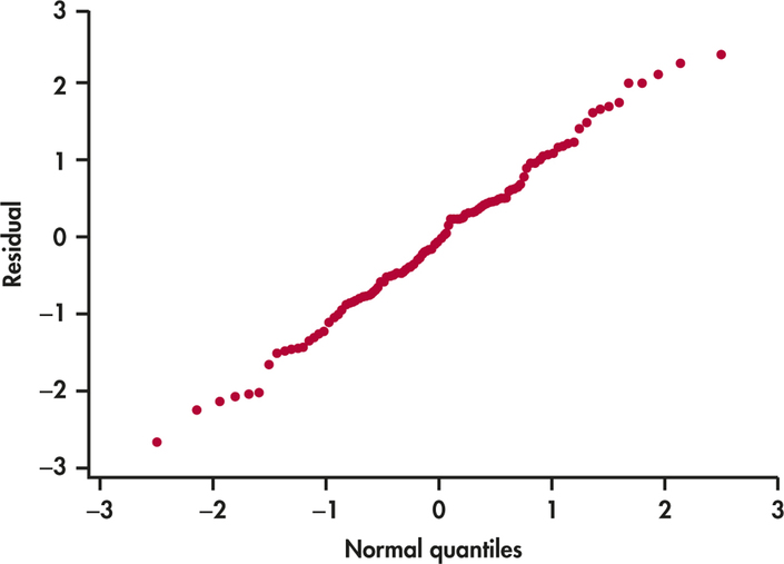
The final condition is that the response varies Normally about the population regression line. In that case, we expect the residuals ei to also be Normally distributed.4 A Normal quantile plot of the residuals (Figure 10.8) shows no serious deviations from a Normal distribution. The data give no reason to doubt the simple linear regression model, so we proceed to inference.
There is no condition that requires Normality for the distributions of the response or explanatory variables. The Normality condition applies only to the distribution of the model deviations, which we assess using the residuals. For the entrepreneur problem, we transformed y to get a more linear relationship as well as residuals that appear Normal with constant variance. The fact that the marginal distribution of the transformed y is more Normal is purely a coincidence.
Confidence intervals and significance tests
Chapter 7 presented confidence intervals and significance tests for means and differences in means. In each case, inference rested on the standard errors of estimates and on t distributions. Inference for the slope and intercept in linear regression is similar in principle. For example, the confidence intervals have the form
estimate±t*SEestimate
where t* is a critical value of a t distribution. It is the formulas for the estimate and standard error that are different.
Confidence intervals and tests for the slope and intercept are based on the sampling distributions of the estimates b1 and b0. Here are some important facts about these sampling distributions:
- When the simple linear regression model is true, each of b0 and b1 has a Normal distribution.
- The mean of b0 is β0 and the mean of b1 is β1. That is, the intercept and slope of the fitted line are unbiased estimators of the intercept and slope of the population regression line.
- The standard deviations of b0 and b1 are multiples of the model standard deviation σ. (We give details later.)
Normality of b0 and b1 is a consequence of Normality of the individual deviations ∈i in the regression model. If the ∈i are not Normal, a general form of the central limit theorem tells us that the distributions of b0 and b1 will be approximately Normal when we have a large sample. Regression inference is robust against moderate lack of Normality. On the other hand, outliers and influential observations can invalidate the results of inference for regression.
Because b0 and b1 have Normal sampling distributions, standardizing these estimates gives standard Normal z statistics. The standard deviations of these estimates are multiples of σ. Because we do not know σ, we estimate it by s, the variability of the data about the least-squares line. When we do this, we get t distributions with degrees of freedom n−2, the degrees of freedom of s. We give formulas for the standard errors SEb1 and SEb0 in Section 10.3. For now, we concentrate on the basic ideas and let software do the calculations.
Inference for Regression Slope
A level C confidence interval for the slope β1 of the population regression line is
b1±t*SEb1
In this expression, t* is the value for the t(n−2) density curve with area C between −t* and t*. The margin of error is m=t*SEb1.
To test the hypothesis H0:β1=0, compute the t statistic
t=b1SEb1
The degrees of freedom are n−2. In terms of a random variable T having the t(n−2) distribution, the P-value for a test of H0 against
Ha:β1>0 is P(T≥t)
Ha:β1<0 is P(T≤t)
Ha:β1≠0 is 2P(T≥|t|)
Formulas for confidence intervals and significance tests for the intercept β0 are exactly the same, replacing b1 and SEb1 by b0 and its standard error SEb0. Although computer outputs often include a test of H0:β0=0, this information usually has little practical value. From the equation for the population regression line, μy=β0+β1x, we see that β0 is the mean response corresponding to x=0. In many practical situations, this subpopulation does not exist or is not interesting.
On the other hand, the test of H0:β1=0 is quite useful. When we substitute β1=0 in the model, the x term drops out and we are left with
μy=β0
This model says that the mean of y does not vary with x. In other words, all the y’s come from a single population with mean β0, which we would estimate by ˉy. The hypothesis H0:β1=0, therefore, says that there is no straight-line relationship between y and x and that linear regression of y on x is of no value for predicting y.
EXAMPLE 10.5 Does Log Income Increase with Education?
entre
CASE 10.1 The Excel regression output in Figure 10.5 (page 492) for the entrepreneur problem contains the information needed for inference about the regression coefficients. You can see that the slope of the least-squares line is b1=0.1126 and the standard error of this statistic is SEb1=0.046116.
Given that the response y is on the log scale, this slope approximates the percent change in y for a unit change in x (see Example 13.10 [pages 661–662] for more details). In this case, one extra year of education is associated with an approximate 11.3% increase in income.
The t statistic and P-value for the test of H0:β1=0 against the two-sided alternative Ha:β1≠0 appear in the columns labeled “t Stat” and “P-value.” The t statistic for the significance of the regression is
t=b1SEb1=0.11260.046116=2.44
and the P-value for the two-sided alternative is 0.0164. If we expected beforehand that income rises with education, our alternative hypothesis would be one-sided, Ha:β1>0. The P-value for this Ha is one-half the two-sided value given by Excel; that is, P=0.0082. In both cases, there is strong evidence that the mean log income level increases as education increases.
A 95% confidence interval for the slope β of the regression line in the population of all entrepreneurs in the United States is
This interval contains only positive values, suggesting an increase in log income for an additional year of schooling. We’re 95% confident that the average increase in income for one additional year of education is between 2.1% and 20.4%.
The distribution for this problem has degrees of freedom. Table D has no entry for 98 degrees of freedom, so we use the table entry for 80 degrees of freedom. As a result, our confidence interval agrees only approximately with the more accurate software result. Note that using the next lower degrees of freedom in Table D makes our interval a bit wider than we actually need for 95% confidence. Use this conservative approach when you don’t know for the exact degrees of freedom.
In this example, we can discuss percent change in income for a unit change in education because the response variable is on the log scale and is not. In business and economics, we often encounter models in which both variables are on the log scale. In these cases, the slope approximates the percent change in for a 1% change in . This is known as elasticity, which is a very important concept in economic theory.
elasticity
Apply Your Knowledge
Treasury bills and inflation.
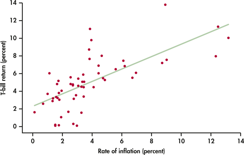
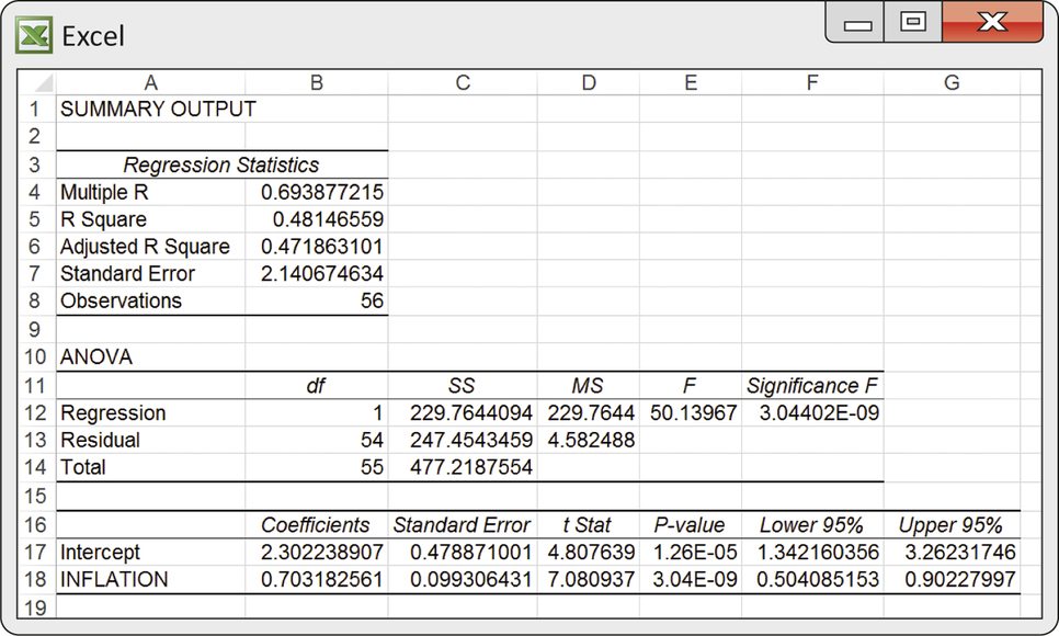
When inflation is high, lenders require higher interest rates to make up for the loss of purchasing power of their money while it is loaned out. Table 10.1 displays the return of six-month Treasury bills (annualized) and the rate of inflation as measured by the change in the government’s Consumer Price Index in the same year.5 An inflation rate of 5% means that the same set of goods and services costs 5% more. The data cover 55 years, from 1958 to 2013. Figure 10.9 is a scatterplot of these data. Figure 10.10 shows Excel regression output for predicting T-bill return from inflation rate. Exercises 10.6 through 10.8 ask you to use this information.
| Year | T-bill percent |
Inflation percent |
Year | T-bill percent |
Inflation percent |
Year | T-bill percent |
Inflation percent |
|---|---|---|---|---|---|---|---|---|
| 1958 | 3.01 | 1.76 | 1977 | 5.52 | 6.70 | 1996 | 5.08 | 3.32 |
| 1959 | 3.81 | 1.73 | 1978 | 7.58 | 9.02 | 1997 | 5.18 | 1.70 |
| 1960 | 3.20 | 1.36 | 1979 | 10.04 | 13.20 | 1998 | 4.83 | 1.61 |
| 1961 | 2.59 | 0.67 | 1980 | 11.32 | 12.50 | 1999 | 4.75 | 2.68 |
| 1962 | 2.90 | 1.33 | 1981 | 13.81 | 8.92 | 2000 | 5.90 | 3.39 |
| 1963 | 3.26 | 1.64 | 1982 | 11.06 | 3.83 | 2001 | 3.34 | 1.55 |
| 1964 | 3.68 | 0.97 | 1983 | 8.74 | 3.79 | 2002 | 1.68 | 2.38 |
| 1965 | 4.05 | 1.92 | 1984 | 9.78 | 3.95 | 2003 | 1.05 | 1.88 |
| 1966 | 5.06 | 3.46 | 1985 | 7.65 | 3.80 | 2004 | 1.58 | 3.26 |
| 1967 | 4.61 | 3.04 | 1986 | 6.02 | 1.10 | 2005 | 3.39 | 3.42 |
| 1968 | 5.47 | 4.72 | 1987 | 6.03 | 4.43 | 2006 | 4.81 | 2.54 |
| 1969 | 6.86 | 6.20 | 1988 | 6.91 | 4.42 | 2007 | 4.44 | 4.08 |
| 1970 | 6.51 | 5.57 | 1989 | 8.03 | 4.65 | 2008 | 1.62 | 0.09 |
| 1971 | 4.52 | 3.27 | 1990 | 7.46 | 6.11 | 2009 | 0.28 | 2.72 |
| 1972 | 4.47 | 3.41 | 1991 | 5.44 | 3.06 | 2010 | 0.20 | 1.50 |
| 1973 | 7.20 | 8.71 | 1992 | 3.54 | 2.90 | 2011 | 0.10 | 2.96 |
| 1974 | 7.95 | 12.34 | 1993 | 3.12 | 2.75 | 2012 | 0.13 | 1.74 |
| 1975 | 6.10 | 6.94 | 1994 | 4.64 | 2.67 | 2013 | 0.09 | 1.50 |
| 1976 | 5.26 | 4.86 | 1995 | 5.56 | 2.54 |
Question 10.6
10.6 Look at the data.
Give a brief description of the form, direction, and strength of the relationship between the inflation rate and the return on Treasury bills. What is the equation of the least-squares regression line for predicting T-bill return?
inflat
Question 10.7
10.7 Is there a relationship?
What are the slope of the fitted line and its standard error? Use these numbers to test by hand the hypothesis that there is no straight-line relationship between inflation rate and T-bill return against the alternative that the return on T-bills increases as the rate of inflation increases. State the hypotheses, give both the statistic and its degrees of freedom, and use Table D to approximate the -value. Then compare your results with those given by Excel. (Excel’s -value 3.04E-09 is shorthand for 0.00000000304. We would report this as “.”)
10.7
. The results are the same as Excel’s.
inflat
Question 10.8
10.8 Estimating the slope.
Using Excel’s values for and its standard error, find a 95% confidence interval for the slope of the population regression line. Compare your result with Excel’s 95% confidence interval. What does the confidence interval tell you about the change in the T-bill return rate for a 1% increase in the inflation rate?
inflat
The word “regression”
To “regress” means to go backward. Why are statistical methods for predicting a response from an explanatory variable called “regression”? Sir Francis Galton (1822–1911) was the first to apply regression to biological and psychological data. He looked at examples such as the heights of children versus the heights of their parents. He found that the taller-than-average parents tended to have children who were also taller than average, but not as tall as their parents. Galton called this fact “regression toward mediocrity,” and the name came to be applied to the statistical method. Galton also invented the correlation coefficient and named it “correlation.”
Why are the children of tall parents shorter on the average than their parents? The parents are tall in part because of their genes. But they are also tall in part by chance. Looking at tall parents selects those in whom chance produced height. Their children inherit their genes, but not their good luck. As a group, the children are taller than average (genes), but their heights vary by chance about the average, some upward and some downward. The children, unlike the parents, were not selected because they were tall and thus, on average, are shorter. A similar argument can be used to describe why children of short parents tend to be taller than their parents.
Here’s another example. Students who score at the top on the first exam in a course are likely to do less well on the second exam. Does this show that they stopped studying? No—they scored high in part because they knew the material but also in part because they were lucky. On the second exam, they may still know the material but be less lucky. As a group, they will still do better than average but not as well as they did on the first exam. The students at the bottom on the first exam will tend to move up on the second exam, for the same reason.
The regression fallacy is the assertion that regression toward the mean shows that there is some systematic effect at work: students with top scores now work less hard, or managers of last year’s best-performing mutual funds lose their touch this year, or heights get less variable with each passing generation as tall parents have shorter children and short parents have taller children. The Nobel economist Milton Friedman says, “I suspect that the regression fallacy is the most common fallacy in the statistical analysis of economic data.”6 Beware.
regression fallacy
Apply Your Knowledge
Question 10.9
10.9 Hot funds?
Explain carefully to a naive investor why the mutual funds that had the highest returns this year will as a group probably do less well relative to other funds next year.
10.9
The mutual funds that had the highest returns this year were high in part because they did well but also in part because they were lucky, so we might expect them to do well again next year but probably not as well as this year.
Question 10.10
10.10 Mediocrity triumphant?
In the early 1930s, a man named Horace Secrist wrote a book titled The Triumph of Mediocrity in Business. Secrist found that businesses that did unusually well or unusually poorly in one year tended to be nearer the average in profitability at a later year. Why is it a fallacy to say that this fact demonstrates an overall movement toward “mediocrity”?
Inference about correlation
The correlation between log income and level of education for the 100 entrepreneurs is . This value appears in the Excel output in Figure 10.5 (page 492), where it is labeled “Multiple R.”7 We might expect a positive correlation between these two measures in the population of all entrepreneurs in the United States. Is the sample result convincing evidence that this is true?
This question concerns a new population parameter, the population correlation. This is the correlation between the log income and level of education when we measure these variables for every member of the population. We call the population correlation , the Greek letter rho. To assess the evidence that in the population, we must test the hypotheses
population correlation
It is natural to base the test on the sample correlation . Table G in the back of the book shows the one-sided critical values of . To use software for the test, we exploit the close link between correlation and the regression slope. The population correlation is zero, positive, or negative exactly when the slope of the population regression line is zero, positive, or negative. In fact, the statistic for testing also tests . What is more, this statistic can be written in terms of the sample correlation .
Test for Zero Population Correlation
To test the hypothesis that the population correlation is 0, compare the sample correlation with critical values in Table G or use the statistic for regression slope.
The statistic for the slope can be calculated from the sample correlation :
This statistic has degrees of freedom.
EXAMPLE 10.6 Correlation between Log Income and Years of Education
CASE 10.1 The sample correlation between log income and education level is from a sample of size . We can use Table G to test
For the row , we find that the -value for lies between 0.005 and 0.01.
We can get a more accurate result from the Excel output in Figure 10.5 (page 492). In the “EDUC” line, we see that with two-sided -value 0.0164. That is, for our one-sided alternative.
Finally, we can calculate directly from as follows:
If we are not using software, we can compare with critical values from the table (Table D) with 80 (largest row less than or equal to ) degrees of freedom.
The alternative formula for the test statistic is convenient because it uses only the sample correlation and the sample size . Remember that correlation, unlike regression, does not require the distinction between explanatory and response variables. For variables and , there are two regressions ( on and on ) but just one correlation. Both regressions produce the same statistic.
The distinction between the regression setting and correlation is important only for understanding the conditions under which the test for 0 population correlation makes sense. In the regression model, we take the values of the explanatory variable as given. The values of the response are Normal random variables, with means that are a straight-line function of . In the model for testing correlation, we think of the setting where we obtain a random sample from a population and measure both and . Both are assumed to be Normal random variables. In fact, they are taken to be jointly Normal. This implies that the conditional distribution of for each possible value of is Normal, just as in the regression model.
jointly Normal
Apply Your Knowledge
Question 10.11
10.11 T-bills and inflation.
We expect the interest rates on Treasury bills to rise when the rate of inflation rises and fall when inflation falls. That is, we expect a positive correlation between the return on T-bills and the inflation rate.
- Find the sample correlation for the 55 years in Table 10.1 in the Excel output in Figure 10.10. Use Table G to get an approximate -value. What do you conclude?
- From , calculate the statistic for testing correlation. What are its degrees of freedom? Use Table D to give an approximate -value. Compare your result with the -value from (a).
- Verify that your for correlation calculated in part (b) has the same value as the for slope in the Excel output.
10.11
(a) . There is a significant positive correlation between T-bills and inflation rate. (b) . The results are the same.
Question 10.12
CASE 10.110.12 Two regressions.
We have regressed the log income of entrepreneurs on their years of education, with the results appearing in Figures 10.5 and 10.6. Use software to regress years of education on log income for the same data.
- What is the equation of the least-squares line for predicting years of education from log income? Is it a different line than the regression line from Figure 10.4? To answer this, plot two points for each equation and draw a line connecting them.
- Verify that the two lines cross at the mean values of the two variables. That is, substitute the mean years of education into the line from Figure 10.5, and show that the predicted log income equals the mean of the log incomes of the 100 subjects. Then substitute the mean log income into your new line, and show that the predicted years of education equals the mean years of education for the entrepreneurs.
- Verify that the two regressions give the same value of the statistic for testing the hypothesis of zero population slope. You could use either regression to test the hypothesis of zero population correlation.
entre