10.2 Introduction to VectorsPrinted Page 699
699
OBJECTIVES
When you finish this section, you should be able to:
NOTE
The word vector comes from the Latin word, meaning “to carry.”
Geometrically, a vector is an object that has both magnitude and direction, and is often represented by an arrow pointing in the direction of the vector. The length of the arrow represents the magnitude of the vector.
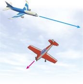
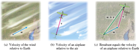
Velocity is a vector. The velocity of an airplane can be represented by an arrow that points in the direction of its flight; the length of the arrow represents its speed (the magnitude of the velocity). See Figure 9. If the airplane speeds up, the length of the arrow increases.
When working with vectors, we refer to real numbers as scalars. Scalars are quantities that have magnitude, but no direction. Physical examples of scalar quantities are time, mass, temperature, and speed.
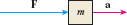
Force and acceleration are also vectors. If a force F is exerted on an object of mass m, the force causes the object to accelerate in the direction of the force. See Figure 10. If a is the acceleration, then F and a are related by the equation F=ma.
1 Represent Vectors GeometricallyPrinted Page 699
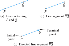
Vectors are closely related to the geometric idea of a directed line segment. If P and Q are distinct points, there is exactly one line containing both P and Q. See Figure 11(a). The points P and Q, and those on the line between P and Q form the line segment ¯PQ. See Figure 11(b). If the points are ordered so they begin with P and end with Q, then we have a directed line segment from P to Q, denoted by →PQ. For the directed line segment →PQ, the point P is the initial point and the point Q is the terminal point. See Figure 11(c).
NOTE
In print, boldface letters are used to denote vectors, to distinguish them from scalars. For handwritten work, an arrow is placed over a letter to denote a vector.
The magnitude of the directed line segment →PQ is the distance from the point P to the point Q; that is, it is the length of the line segment ¯PQ. The direction of →PQ is from P to Q. If a vector v has the same magnitude and the same direction as the directed line segment →PQ, then \bbox[5px, border:1px solid black, #F9F7ED]{ \mathbf{v}=\overrightarrow{\it PQ}}
The vector whose magnitude is 0 is called the zero vector \mathbf{0}. The zero vector is assigned no direction.
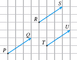
Two vectors \mathbf{v} and \mathbf{w} are equal, written \mathbf{v}=\mathbf{w}, if they have the same magnitude and the same direction. For example, the vectors in Figure 12 are equal even though they have different initial points and terminal points.
700
As a result, it is useful to think of a vector simply as an arrow, keeping in mind that two arrows (vectors) are equal if they have the same direction and the same length (magnitude).
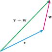
Since location does not affect a vector, we add two vectors \mathbf v and \mathbf w by positioning vector \mathbf{w} so that its initial point coincides with the terminal point of \mathbf{v}. The vector sum \mathbf{v}+\mathbf{w} is the unique vector represented by the arrow from the initial point of \mathbf{v} to the terminal point of \mathbf{w}, as shown in Figure 13.
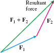
We said that forces can be represented by vectors. But how do we know that forces “add” the same way vectors do? Well, physicists say they do, and laboratory experiments bear it out. So if \mathbf{F}_{1} and \mathbf{F} _{2} are two forces simultaneously acting on an object, the vector sum \mathbf{F}_{1}\,\mathbf{+\,F}_{2} is equal to the force that produces the same effect as that obtained when the forces \mathbf{F}_{1} and \mathbf{F} _{2} are applied at the same time to the same object. The force \mathbf{F} _{1}+\mathbf{F}_{2} is called the resultant force. See Figure 14.
NOW WORK
If \mathbf{w} is a vector describing the velocity of the wind relative to Earth and if \mathbf{v} is a vector describing the velocity of an airplane in the air, then \mathbf{w}+\mathbf{v} is a vector describing the velocity of the airplane relative to Earth. See Figure 15.
EXAMPLE 1Graphing a Resultant Vector
A swimmer swims at a constant speed of 3 miles per hour (mi/h) and heads directly across a river whose current is 4 mi/h.
- (a) Draw vectors representing the swimmer and the current.
- (b) Draw the resultant vector.
- (c) Interpret the result.
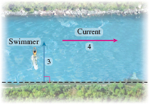
Solution (a) We represent the swimmer by a vector pointing directly across the river and the current by a vector pointing parallel to a straight shore line. Since the swimmer’s speed is 3 \,\rm{mi/h}, and the current’s speed is 4 \,\rm{mi/h}, the length of the vector representing the swimmer is 3 units, and the length of the vector representing the current is 4 units. See Figure 16.
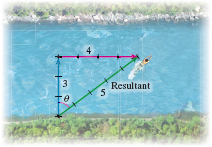
(b) The resultant vector is the sum of the vectors in (a). See Figure 17.
(c) The resultant vector shows the true speed of the swimmer and true direction of the swim. In fact, the true speed is 5 \,\rm{mi/h} and the true direction can be described in terms of the angle \theta as \theta =\tan ^{-1}\dfrac{4}{3}\approx 53.1^{\circ}.
NOW WORK
Next, we examine properties of vectors. Many of these properties are similar to properties of real numbers.
Properties of Vector AdditionPrinted Page 701
701


Let \mathbf{u}, \mathbf{v}, and \mathbf{w} represent any three vectors.
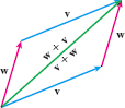
- Commutative property of vector addition (Figure 18): \bbox[5px, border:1px solid black, #F9F7ED]{ \mathbf{w+v=v}+\mathbf{w}}
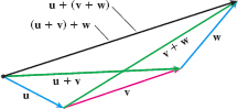
- Associative property of vector addition (Figure 19): \bbox[5px, border:1px solid black, #F9F7ED]{ \mathbf{u}+ (\mathbf{v+w}) =( \mathbf{u}+\mathbf{v}) +\mathbf{w}}
- Additive identity property The zero vector \mathbf{0} is called the additive identity. The sum of any vector \mathbf{v } and the zero vector \mathbf{0} equals \mathbf{v}. \bbox[5px, border:1px solid black, #F9F7ED]{ \mathbf{v+0=0}+\mathbf{v=v}} \def\sf{\bm 0}
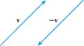
- Additive inverse property For any vector \mathbf{ v}, the vector -\mathbf{v}, called the additive inverse of \mathbf{v}, has the same magnitude as \mathbf{v}, but the opposite direction, as shown in Figure 20. The sum of \mathbf{v} and its additive inverse -\mathbf{v} is the zero vector \mathbf{0}. \bbox[5px, border:1px solid black, #F9F7ED]{ \mathbf{v+}(-\mathbf{v}) = (-\mathbf{v}) + \mathbf{v=0}}
DEFINITION Difference of Two vectors
The difference of two vectors \mathbf{v}-\mathbf{w} is defined as \bbox[5px, border:1px solid black, #F9F7ED]{ \mathbf{v}-\mathbf{w}=\mathbf{v} + (-\mathbf{w})}
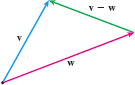
The difference \mathbf{v}-\mathbf{w} between two vectors can be obtained by positioning \mathbf{v} and \mathbf{w} so their initial points coincide. Then the vector from the terminal point of \mathbf{w} to the terminal point of \mathbf{v} is the difference \mathbf{v}-\mathbf{w}, as shown in Figure 21.
The product of a vector \mathbf{v} and a scalar a produces a vector called the scalar multiple of \mathbf{v}.
DEFINITION Scalar Multiple
If a is a scalar and \mathbf{v} is a vector, the product a \mathbf{v}, called a scalar multiple of \mathbf{v}, is the vector with magnitude \left\vert a\right\vert times the magnitude of \mathbf{v}, in the same direction as \mathbf{v} when a\gt 0 and in the opposite direction from \mathbf{v} when a\lt 0.
If either a=0 or \mathbf{v=0}, then a\mathbf{v=0}.
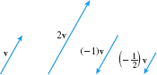
See Figure 22 for illustrations of scalar multiples of \mathbf{v}. Notice that the additive inverse of \mathbf{v} can be represented as the scalar multiple ( -1) \mathbf{v}.
We saw earlier that if \mathbf{a} is the acceleration of an object of mass m due to a force \mathbf{F} being exerted, then by Newton’s second law of motion, \mathbf{F}=m\mathbf{a}. Here, m\mathbf{a} is the product of the scalar m and the vector \mathbf{a}.
Scalar multiples have the following properties:
Properties of Scalar Multiplication
If \mathbf{v} and \mathbf{w} are any two vectors and \mathbf 0 is the zero vector, then:
- 0{\mathbf v} = \mathbf{0}
- 1{\mathbf v} = \mathbf{v}
- (-1) \mathbf{v} = \mathbf{-v}
- (a + b) \mathbf{v} = a{\mathbf v} + b{\mathbf v}
- {a} (\mathbf{v + w}) = a{\mathbf v} + a{\mathbf w}
- {a}(b{\mathbf v}) = ({ab})\mathbf{v}
2 Use Properties of VectorsPrinted Page 702
702

EXAMPLE 2Using Properties of Vectors
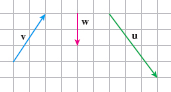
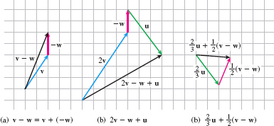
Use the vectors illustrated in Figure 23 to graph each of the following vectors:
- (a) \mathbf{v}-\mathbf{w}
- (b) 2\mathbf{v}-\mathbf{w}+\mathbf{u}
- (c) \dfrac{2}{3}\mathbf{u}+\dfrac{1}{2}(\mathbf{v}-\mathbf{w})
Solution We reposition the vectors in Figure 23 as shown in Figure 24 to graph the desired vectors.