3.5 Taylor PolynomialsPrinted Page 240
240

In the last section, we found that if a function f is differentiable in an interval (a,b), then a linear approximation L(x) to f at a number x0 in the interval is given by L(x)=f(x0)+f′(x0)(x−x0)
where y=L(x) is the tangent line to the graph of f at the point (x0,f(x0)). This approximation for f is good if x is close enough to x0, but as the interval widens, the accuracy of the estimate decreases.
The linear approximation y=L(x) is a first degree polynomial function. If the function f has derivatives of orders 1 to n at x0, then a polynomial function Pn(x) of degree n can be used to approximate f near x0.
ORIGINS
The Taylor polynomial is named after the English mathematician Brook Taylor (1685–1731). Taylor grew up in an affluent but strict home. He was home-schooled in the arts and the classics until he attended Cambridge University in 1703, where he studied mathematics. He was an accomplished musician and painter as well as a mathematician.
To be sure that the polynomial approximation Pn(x) fits f well, we require: Pn(x0)=f(x0)P′n(x0)=f′(x0)P′′n(x0)=f′′(x0)…P(n)n(x0)=f(n)(x0)
That is, the value at x0 of the function f and its first n derivatives equals the value at x0 of the polynomial approximation and its first n derivatives.
DEFINITION Taylor Polynomial
If a function f and its first n derivatives are defined on an interval containing the number x0, then \bbox[5px, border:1px solid black, #F9F7ED]{P_{n}( x) =f( x_{0}) +f^\prime ( x_{0}) ( x-x_{0}) +\dfrac{f^{\prime \prime} ( x_{0}) }{2!}( x-x_{0}) ^{2}+\cdots+\dfrac{f^{( n) }( x_{0}) }{\,n!}( x-x_{0}) ^{n}} is called the nth Taylor Polynomial for f at x_{0}.
NOTE
The sum of the first two terms of a Taylor Polynomial is the linear approximation of f at x. That is, {P}_{1}({x}) = L({x}).
1 Find a Taylor PolynomialPrinted Page 240
EXAMPLE 1Finding a Taylor Polynomial for f( x)=\sqrt{x}
Find the Taylor Polynomial P_{3}( x) for f( x) =\sqrt{x} at 1.
Solution The first three derivatives of f(x) =\sqrt{x} are \begin{eqnarray*} f^\prime ( x) &=&\dfrac{1}{2\sqrt{x}}\qquad\qquad f^{\prime \prime} ( x) =\dfrac{d}{dx}\left( \dfrac{x^{-1/2}}{2}\right) =-\dfrac{1}{4x^{3/2}} \\ f^{\prime \prime \prime} ( x) &=&\dfrac{d}{dx}\left( -\dfrac{x^{-3/2}}{4}\right) =\dfrac{3}{8x^{5/2}} \end{eqnarray*}
Then f(1) =1\qquad f^\prime (1) =\dfrac{1}{2}\qquad f^{\prime \prime} (1) =-\dfrac{1}{4}\qquad f^{\prime \prime \prime} (1) =\dfrac{3}{8}
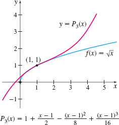
The Taylor Polynomial P_{3}( x) for f( x) =\sqrt{x} at 1 is \begin{eqnarray*} P_{3}( x) &=&f(1) +f^\prime (1) ( x-1) +\dfrac{f^{\prime \prime} (1) }{2!}( x-1) ^{2}+\dfrac{f^{\prime \prime \prime} (1) }{3!}( x-1)^{3}\\ &=&1+\dfrac{x-1}{2}-\dfrac{( x-1) ^{2}}{8}+\dfrac{( x-1) ^{3}}{16} \end{eqnarray*}
The graphs of the function f and the Taylor Polynomial P_{3} are shown in Figure 17. Notice how P_{3}( x) \approx f( x) for values of x near 1.
NOW WORK
241
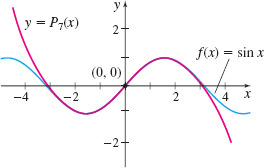
EXAMPLE 2Finding a Taylor Polynomial for f( x) =\sin x
Find the Taylor Polynomial P_{7}( x) for f( x) =\sin x at 0.
Solution The derivatives of f( x) =\sin x at 0 are \begin{array}{rcl@{\qquad}rcl@{\qquad}rcl@{\qquad}rcl} f( x) &=&\sin x & f^\prime ( x) &=&\cos x & f^{\prime \prime} ( x) &=&-\!\sin x & f^{\prime \prime \prime} ( x) &=&-\!\cos x \\ f( 0) &=&0 & f^\prime ( 0) &=&1 & f^{\prime \prime} ( 0) &=&0 & f^{\prime \prime \prime} ( 0) &=&-1 \\ f^{( 4) }( x) &=&\sin x & f^{(5) }( x) &=&\cos x & f^{( 6)}( x) &=&-\!\sin x & f^{( 7) }( x) &=&-\!\cos x \\ f^{( 4) }( 0) &=&0 & f^{(5) }( 0) &=&1 & f^{( 6) }( 0) &=&0 & f^{( 7) }( 0) &=&-1 \end{array}
The Taylor Polynomial P_{7}( x) for \sin x at 0 is P_{7}( x) =f( 0) +f^\prime ( 0) x+\dfrac{f^{\prime \prime} ( 0) }{2!}x^{2}+\dfrac{f^{\prime\prime \prime} ( 0) }{3!}x^{3}+\cdots +\dfrac{f^{( 7) }( 0) }{7!}x^{7}=x-\dfrac{x^{3}}{3!}+\dfrac{x^{5}}{5!}-\dfrac{x^{7}}{7!}
Figure 18 shows the graph of P_{7} superimposed on the graph of y=\sin x.
NOW WORK

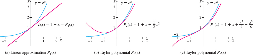
EXAMPLE 3Finding a Taylor Polynomial for f( x) =e^{x}
Find the Taylor Polynomial P_{n}( x) for f( x) =e^{x} at 0.
Solution The derivatives of f( x) =e^{x} are \begin{array}{rcl@{\qquad}rcl@{\qquad}rcl@{\qquad}rcl@{ }c@{ }rcl} f( x) = e^{x} & f^\prime ( x) = e^{x} & f^{\prime \prime} ( x) = e^{x} & f^{\prime \prime \prime} ( x) = e^{x} & \ldots & f^{( n) }( x) = e^{x} \\ f( 0) = 1 & f^\prime ( 0) = 1 & f^{\prime \prime} ( 0) = 1 & f^{\prime \prime \prime} ( 0) = 1 & \ldots & f^{( n)}( 0) = 1 \end{array}
The Taylor Polynomial P_{n}( x) at 0 is \begin{eqnarray*} P_{n}( x) &=&f( 0) +f^\prime ( 0) x+\dfrac{ f^{\prime \prime} ( 0) }{2!}x^{2}+\dfrac{f^{\prime \prime\prime} ( 0) }{3!}x^{3}+\cdots +\dfrac{f^{( n) }( 0) }{n!}x^{n}\\ &=&1+x+\dfrac{x^{2}}{2!}+\dfrac{x^{3}}{3!}+\cdots +\dfrac{ x^{n}}{n!} \end{eqnarray*}
NOTE
In Chapter 8 we investigate the relationship between a function f and its Taylor Polynomials.
Figure 19 illustrates how the graphs of the Taylor Polynomials P_{1}( x) , P_{2}( x) , and P_{3}( x) compare to the graph of f( x) =e^{x} near 0.