5.3 The Fundamental Theorem of CalculusPrinted Page 362
362
In this section, we discuss the Fundamental Theorem of Calculus, a method for finding integrals more easily, avoiding the need to find the limit of Riemann sums. The Fundamental Theorem is aptly named because it links the two branches of calculus: differential calculus and integral calculus. As it turns out, the Fundamental Theorem of Calculus has two parts, each of which relates an integral to an antiderivative.
Suppose f is a function that is continuous on a closed interval [a,b]. Then the definite integral ∫baf(x)dx exists and is equal to a real number. Now if x denotes any number in [a,b], the definite integral ∫xaf(t)dt exists and depends on x. That is, ∫xaf(t)dt is a function of x, which we name I, for “integral.” I(x)=∫xaf(t)dt
NEED TO REVIEW?
Antiderivatives are discussed in Section 4.8, pp. 328-331.
The domain of I is the closed interval [a,b]. The integral that defines I has a variable upper limit of integration x. The t that appears in the integrand is a dummy variable. Surprisingly, when we differentiate I with respect to x, we get back the original function f. That is, ∫xaf(t)dt is an antiderivative of f.
THEOREM Fundamental Theorem of Calculus, Part 1
Let f be a function that is continuous on a closed interval [a,b]. The function I defined by \bbox[5px, border:1px solid black, #F9F7ED]{\bbox[5pt]{ I\,(x)=\int_{a}^{x}f(t)\,dt } }
has the properties that it is continuous on [a,b] and differentiable on (a,b). Moreover, \bbox[5px, border:1px solid black, #F9F7ED]{\bbox[5pt]{ I' (x)=\dfrac{d}{dx}\left[\int_{a}^{x}f(t)\,dt \right] =f(x) } }
for all x in (a,b).
The proof of Part 1 of the Fundamental Theorem of Calculus is given in Appendix B. However, if the integral \int_{a}^{x}f(t)\, dt represents area, we can interpret the theorem using geometry.
Figure 22 shows the graph of a function f that is nonnegative and continuous on a closed interval [a,b] . Then I(x) =\int_{a}^{x}f(t)\, dt equals the area under the graph of f from a to x.
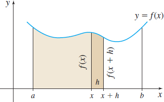
\begin{eqnarray} I(x) =\int_{a}^{x}f(t) \,dt &=& \hbox{the area under the graph of } f \hbox{ from } a \hbox{ to } x \nonumber \\ I(x+h) =\int_{a}^{x+h}f(t) \,dt &=& \hbox{the area under the graph of } f \hbox{ from } a \hbox{ to } x+h \nonumber\\ I(x+h) -I(x) &=& \hbox{the area under the graph of } f \hbox{ from } x \hbox{ to } x+h \nonumber\\ \dfrac{I(x+h) -I(x)}{h} &=& \dfrac{\hbox{the area under the graph of }f \hbox{ from } x \hbox{ to } x+h} {h}\qquad \end{eqnarray}
363
Based on the definition of a derivative, \begin{equation} \ \lim\limits_{h\rightarrow 0}\left[ \dfrac{I(x+h) -I(x) }{h}\right] =I^\prime (x) \end{equation}
Since f is continuous, \lim\limits_{h\rightarrow 0}f(x+h) =f(x) . As h\rightarrow 0, the area under the graph of f from x to x+h gets closer to the area of a rectangle with width h and height f(x). That is, \begin{equation} \lim\limits_{h\rightarrow 0}\dfrac{\hbox{the area under the graph of }f \hbox{ from }x\hbox{ to }x+h}{h}=\lim\limits_{h\rightarrow 0}\dfrac{h[ f(x) ] }{h}=f(x) \end{equation}
Combining (1), (2), and (3), it follows that I^\prime (x) =f(x).
1 Use Part 1 of the Fundamental Theorem of CalculusPrinted Page 363
EXAMPLE 1Using Part 1 of the Fundamental Theorem of Calculus
(a) \dfrac{d}{dx}\int_{0}^{x}\sqrt{t+1}\,dt=\sqrt{ x+1}
(b) \dfrac{d}{dx}\int_{2}^{x}\dfrac{s^{3}-1}{2s^{2}+s+1}ds=\dfrac{x^{3}-1}{2x^{2}+x+1}
NOW WORK

EXAMPLE 2Using Part 1 of the Fundamental Theorem of Calculus
Find \dfrac{d}{dx}\int_{4}^{3x^{2}+1}\sqrt{e^{t}+t}\,dt.
NEED TO REVIEW?
The Chain Rule is discussed in Section 3.1, pp. 198-200.
Solution The upper limit of integration is a function of x, so we use the Chain Rule along with Part 1 of the Fundamental Theorem of Calculus.
Let y=\int_{4}^{3x^{2}+1}\sqrt{e^{t}+t}\,dt and u(x) =3x^{2}+1. Then y=\int_{4}^{u}\sqrt{e^{t}+t}\,dt and \begin{eqnarray*} \dfrac{d}{dx}\int_{4}^{3x^{2}+1}\sqrt{e^{t}+t}\,dt &=& \dfrac{dy}{dx} \underset{\underset{{\color{#0066A7}{\hbox{Chain Rule}}}}{\color{#0066A7}{\uparrow}}}{=} \dfrac{dy}{du}\cdot \dfrac{du}{dx}= \left[ \dfrac{d}{du}\int_{4}^{u}\sqrt{e^{t}+t}\,dt\right] \cdot \dfrac{du}{dx} \\ & \underset{\underset{\color{#0066A7}{{\hbox{Use the Fundamental Theorem}}}} {\color{#0066A7}{\uparrow}}}{=}& \sqrt{e^{u}+u}\cdot \dfrac{du}{dx} \underset{\underset{{\color{#0066A7}{{\hbox{\({u=3x}^{2}+1\); \(\dfrac{du}{dx}=6x\)}}}}{\hbox{\( \)}}}{\color{#0066A7}{\uparrow}}}{=}\sqrt{e^{( 3x^{2}+1) }+3x^{2}+1}\cdot 6x \\ \end{eqnarray*}
NOW WORK
EXAMPLE 3Using Part 1 of the Fundamental Theorem of Calculus
Find \dfrac{d}{dx}\int_{x^{3}}^{5}(t^{4}+1)^{1/3}\,dt.
Solution To use Part 1 of the Fundamental Theorem of Calculus, the variable must be part of the upper limit of integration. So, we use the fact that \int_{a}^{b}f(x)\,dx=-\int_{b}^{a}f(x)\,dx to interchange the limits of integration. \dfrac{d}{dx}\int_{x^{3}}^{5}(t^{4}+1)^{1/3}\,dt=\dfrac{d}{dx}\left[ {-} \int_{5}^{x^{3}}(t^{4}+1)^{1/3} dt\right] ={-}\dfrac{d}{dx} \int_{5}^{x^{3}}(t^{4}+1)^{1/3} dt
364
Now we use the Chain Rule. We let y=\int_{5}^{x^{3}}( t^{4}+1)^{1/3}dt and u(x) =x^{3}.
NOTE
In these examples, the differentiation is with respect to the variable that appears in the upper or lower limit of integration and the answer is a function of that variable.
\begin{eqnarray*} \dfrac{d}{dx}\int_{x^{3}}^{5}(t^{4}+1)^{1/3}\,dt &=& -\dfrac{d}{dx}\int_{5}^{x^{3}}(t^{4}+1)^{1/3}\,dt=-\dfrac{dy}{dx} \underset{ \underset{ \color{#0066A7}{\hbox{Chain Rule}} } {\color{#0066A7}{\uparrow}} } {=} -\dfrac{dy}{du}\cdot\dfrac{du}{dx}\\ &=&-\dfrac{d}{du}\int_{5}^{u}( t^{4}+1) ^{1/3}dt\cdot \dfrac{du}{dx} \\ &=& -(u^{4}+1)^{1/3}\cdot \dfrac{du}{dx} {\color{#0066A7}\enspace{\color{#0066A7}{\hbox{Use the Fundamental Theorem}}}} \\ &=&-( x^{12}+1) ^{1/3}\cdot 3x^{2} \enspace{\color{#0066A7}{{\hbox{\({u=x}^{3}\); \(\dfrac{du}{dx}=3x^{2}\)}}}} \\ &=&-3x^{2}(x^{12}+1)^{1/3} \end{eqnarray*}
NOW WORK
Part 1 of the Fundamental Theorem of Calculus establishes a relationship between the derivative and the definite integral. Part 2 of the Fundamental Theorem of Calculus provides a method for finding a definite integral without using Riemann sums.
THEOREM Fundamental Theorem of Calculus, Part 2
Let f be a function that is continuous on a closed interval [a,b]. If F is any antiderivative of f on [a,b], then \bbox[5px, border:1px solid black, #F9F7ED]{\bbox[5pt]{ \int_{a}^{b}f(x)\,dx=F(b)-F(a)}}
Proof
Let I(x) =\int_{a}^{x}f(t)\, dt. Then from Part 1 of the Fundamental Theorem of Calculus, I=I(x) is continuous for a\leq x\leq b and differentiable for a\lt x\lt b. So, \dfrac{d}{dx}\int_{a}^{x}f(t) ~dt=f(x) \qquad a\lt x\lt b
RECALL
Any two antiderivatives of a function differ by a constant.
That is, \int_{a}^{x}f(t)\,dt is an antiderivative of f. So, if F is any antiderivative of f, then F(x)=\int_{a}^{x}f(t)\,dt+C
where C is some constant. Since F is continuous on [a,b] , we have
NOTE
For any constant C, [F(b)+C]-[F(a)+C]=F(b)-F(a). In other words, it does not matter which antiderivative of f is chosen when using Part 2 of the Fundamental Theorem of Calculus, since the same answer is obtained for every antiderivative.
F(a)=\int_{a}^{a}f(t) dt+C \qquad F(b)=\int_{a}^{b}f(t) dt+C
Since, {\int_{a}^{a}{f(t) dt}=0}, subtracting F(a) from F(b) gives F(b)-F(a)=\int_{a}^{b}f(t) dt
Since t is a dummy variable, we can replace t by x and the result follows.
As an aid in computation, we introduce the notation \bbox[5px, border:1px solid black, #F9F7ED]{\bbox[#FAF8ED,5pt]{ \int_{a}^{b}f(x)~dx= \Big[F(x)\Big] _{a}^{b}=F(b)-F(a)}}
The notation \big[F(x)\big] _{a}^{b} also suggests that to find \int_{a}^{b}f(x) \,dx, we first find an antiderivative F(x) of f(x). Then we write \big[F(x)\big]_{a}^{b} to represent F(b)-F(a).
2 Use Part 2 of the Fundamental Theorem of CalculusPrinted Page 365
365
EXAMPLE 4Using Part 2 of the Fundamental Theorem of Calculus
Use Part 2 of the Fundamental Theorem of Calculus to find:
- (a) {\int_{-2}^{1}{x^{2} dx}}
- (b) {\int_{0}^{\pi /6}{\cos x dx}}
- (c) {\int_{0}^{\sqrt{3}/2}}\dfrac{1}{\sqrt{1-x^{2}}}\,{dx}
- (d) {\int_{1}^{2}}\dfrac{1}{x} {dx}
Solution (a) An antiderivative of f(x) =x^{2} is F(x) =\dfrac{x^{3}}{3}. By Part 2 of the Fundamental Theorem of Calculus, {\int_{-2}^{1}{x^{2}}}dx=\left[ {\dfrac{{x^{3}}}{{3}}}\right] _{-2}^{1}={\dfrac{{1}^{3}}{{3}}}-{\dfrac{{\left( {-2}\right) ^{3}}}{{3}}}={\dfrac{{1}}{{3}}}+{\dfrac{{8}}{{3}}}={\dfrac{{9}}{{3}}}=3
(b) An antiderivative of f(x) =\cos x is F(x) =\sin x. By Part 2 of the Fundamental Theorem of Calculus, \int_{0}^{\pi /6}\cos x\,dx= \Big[\sin x\Big] _{0}^{\pi /6}=\sin \dfrac{\pi }{6}-\sin 0=\dfrac{1}{2}
(c) An antiderivative of f(x) =\dfrac{1}{\sqrt{1-x^{2}}} is F(x) =\sin ^{-1}x, provided \vert x\vert \lt1. By Part 2 of the Fundamental Theorem of Calculus, {\int_{0}^{\sqrt{3}/2}} \dfrac{1}{\sqrt{1-x^{2}}}\,dx= \Big[\sin^{-1}x\Big] _{0}^{\sqrt{3}/2}=\sin ^{-1}\dfrac{\sqrt{3}}{2}-\sin ^{-1}0=\dfrac{\pi}{3}-0=\dfrac{\pi}{3}
(d) An antiderivative of f(x)=\dfrac{1}{x} is F(x) =\ln \,\vert x\vert . By Part 2 of the Fundamental Theorem of Calculus, {\int_{1}^{2}} \dfrac{1}{x}\,dx= \Big[\ln \vert x\vert\Big] _{1}^{2}=\ln 2-\ln 1=\ln 2-0=\ln 2
NOW WORK
EXAMPLE 5Finding the Area Under a Graph
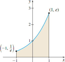
Find the area under the graph of f(x) =e^{x} from -1 to 1.
Solution Figure 23 shows the graph of f(x)=e^{x} on the closed interval [-1,1] .
The area A under the graph of f from -1 to 1 is given by A= \int\nolimits_{-1}^{1}e^{x}\, dx=\Big[e^{x}\Big] _{-1}^{1}=e^{1}-e^{-1} = e-\dfrac{1}{e} \approx 2.35.
NOW WORK
3 Interpret an Integral Using Part 2 of the Fundamental Theorem of CalculusPrinted Page 365
Part 2 of the Fundamental Theorem of Calculus states that, under certain conditions, \int_{a}^{b}f(x)\, dx=F(b) -F(a)\qquad \hbox{where } F^\prime =f
That is, \int_{a}^{b} F^\prime (x)\, dx=F(b) -F(a)
366
In other words, \bbox[5px, border:1px solid black, #F9F7ED]{\bbox[#FAF8ED,5pt]{ \begin{array}{@{\hspace*{-4pt}}lll} &&\hbox{The integral from } a \hbox{ to } b \hbox{ of the rate of change of } F \hbox{ equals the change} \\ &&\hbox{ in } F \hbox{ from } a \hbox{ to } b. \end{array}}}
EXAMPLE 6Interpreting an Integral Whose Integrand Is a Rate of Change
- (a) The function P=P(t) relates the population P (in billions of persons) as a function of the time t (in years). Suppose \int_{0}^{10}P^\prime (t)\, dt=3. Since P^{\prime} (t) is the rate of change of the population with respect to time, then the change in population from t=0 to t=10 is 3 billion persons.
- (b) The function v=v(t) is the speed v (in meters per second) of an object at a time t (in seconds). If \int_{0}^{5}v(t) dt=8, then the object travels 8 m during the interval 0\leq t\leq 5. Do you see why? The speed v=v(t) is the rate of change of distance s with respect to time t. That is, v=\dfrac{ds}{dt}.
This interpretation of an integral is important since it reveals how to go from a rate of change of a function F back to the change itself.