12.3 Partial DerivativesPrinted Page 829
OBJECTIVES
When you finish this section, you should be able to:
- Find the partial derivatives of a function of two variables (p. 829)
- Interpret partial derivatives as the slope of a tangent line (p. 831)
- Interpret partial derivatives as a rate of change (p. 832)
- Find second-order partial derivatives (p. 834)
- Find the partial derivatives of a function of \(n\) variables (p. 836)
1 Find the Partial Derivatives of a Function of Two VariablesPrinted Page 829
Suppose \(z=f(x,y)\) is a function of two variables \(x\) and \(y\). If \(y_{0}\) is a constant, then the function \(z=f(x,y)=f(x,y_{0})\) is a function of the single variable \(x\). If \(z=f(x,y_0)\) is differentiable at \(x=x_{0}\), then the derivative of the function \(f(x,y_{0})\) at \(x_{0}\) is called the partial derivative of \(f\) with respect to \(x\) at \((x_{0},y_{0})\) and is denoted by \(f_{x}(x_{0},y_{0})\).
Similarly, if \(x_{0}\) is a constant, then \(z=f(x_{0},y)\) is a function of the single variable \(y\). If \(z=f(x_0,y)\) is differentiable at \(y=y_{0}\), then its derivative is called the partial derivative of \(f\) with respect to \(y\) at \((x_{0},y_{0})\) and is denoted by \(f_{y}(x_{0}, y_{0})\).
830
DEFINITION Partial Derivatives
Let \(z=f(x,y)\) be a function of two variables, and let \((x,y)\) be any interior point* of the domain of \(f\). The first-order partial derivative of \({\boldsymbol f}\) with respect to \(x\) and the first-order partial derivative of \({\boldsymbol f}\) with respect to \(y\) are functions \(f_{x}\) and \(f_{y}\) defined by \[\bbox[5px, border:1px solid black, #F9F7ED]{\bbox[#FAF8ED,5pt]{ \begin{array}{l} f_{x}(x,y) =\lim\limits_{\Delta x\rightarrow 0}\dfrac{f( x+\Delta x,y) -f(x,y) }{\Delta x} \\ f_{y}(x,y) =\lim\limits_{\Delta y\rightarrow 0}\dfrac{f( x,y+\Delta y) -f(x,y) }{\Delta y} \end{array}}} \]
provided these limits exist.
*Although partial derivatives may be defined at boundary points of the domain of \(f\), they are more difficult to handle and are not discussed in this book.
NEED TO REVIEW?
The definition of the derivative is discussed in Section 2.2, p. 154.
Observe the similarity between the definitions of partial derivatives above and the definition of a derivative as the limit of a difference quotient given in Chapter 2. Namely, if \(y=f(x)\), then \(f' (x) =\lim\limits_{h\rightarrow 0}\dfrac{f( x+h) -f(x) }{h}\). In \(f_{x}(x,y)\), the increment \(\Delta x\) applies to \(x\), while \(y\) is treated as a constant, and in \(f_{y}(x,y)\), the increment \( \Delta y\) applies to \(y\), while \(x\) is treated as a constant.
IN WORDS
We find the partial derivative of \(f\) with respect to \(x\) by differentiating \(f\) with respect to \(x\) while treating \(y\) as if it were a constant.
We find the partial derivative of \(f\) with respect to \(y\) by differentiating \(f\) with respect to \(y\) while treating \(x\) as if it were a constant.
Just as the derivative of a function \(y=f(x)\) is itself a function, the partial derivatives \(f_{x}\) and \(f_{y}\) of a function \(z=f(x,y)\) are functions, generally of two variables.
The Sum, Difference, Product, and Quotient Rules used for finding the derivative of a function \(f\) of one variable also are used to find partial derivatives.
EXAMPLE 1Finding the Partial Derivatives of a Function of Two Variables
For each function \(z=f(x,y)\), find \(f_{x}(x,y)\) and \(f_{y}(x,y)\).
- (a) \(f(x,y)=3x^{2}y+2x-3y\)
- (b) \(f(x,y)=x\;\sin\;y+y\;\sin\;x\)
Solution (a) To find \(f_{x}(x,y)\), treat \(y\) as a constant in \( f(x,y)=3x^{2}y+2x-3y\) and differentiate with respect to \(x\). The result is \[ f_{x}(x,y)=6\;xy+2 \]
To find \(f_{y}(x,y)\), treat \(x\) as a constant and differentiate with respect to \(y\). The result is \[ f_{y}(x,y)=3x^{2}-3 \]
(b) For \(f(x,y)=x\;\sin\;y+y\;\sin\;x\), we have 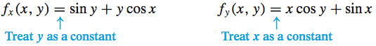
NOW WORK
EXAMPLE 2Finding the Partial Derivatives of a Function at a Point \(( x_{0},y_{0})\)
For \(f(x,y)=x\;\sin\;y+y\;\sin\;x\), find \(f_{x}\left(\dfrac{\pi }{3},\dfrac{\pi }{ 6}\right)\) and \(f_{y}\left( \dfrac{\pi }{3},\dfrac{\pi }{6}\right)\).
Solution We use the results from Example 1(b): \[ \begin{eqnarray*} f_{x}(x,y) &=&\sin\;y+y\;\cos\;x\\[3pt] f_{x}\left( \dfrac{\pi }{3},\dfrac{\pi }{6}\right) &=&\sin \dfrac{\pi }{6}+\dfrac{\pi }{6}\cos \dfrac{\pi }{3}=\dfrac{1}{2}+\dfrac{\pi }{6}\left( \dfrac{1}{2}\right) =\dfrac{6+\pi }{12}\\ f_{y}(x,y)&=&x\;\cos\;y+\;\sin\;x\\[3pt] f_{y}\left( \dfrac{\pi }{3},\dfrac{\pi }{6}\right) &=&\dfrac{\pi }{3}\cos \dfrac{\pi }{6}+\sin \dfrac{\pi }{3}=\dfrac{\pi }{3}\left( \dfrac{\sqrt{3}}{2}\right) +\dfrac{\sqrt{3}}{2 }=\dfrac{( \pi +3) \sqrt{3}}{6} \end{eqnarray*} \]
831
Another Notation
Another notation used for the partial derivatives of a function \(z=f(x,y)\) is \[ f_{x}(x, y)=\frac{\partial f}{\partial x}=\frac{\partial z}{\partial x}\qquad \hbox{and}\qquad f_{y}(x, y)=\frac{\partial f}{\partial y}=\frac{\partial z}{\partial y} \]
The symbols \(\dfrac{\partial }{\partial x}\) and \(\dfrac{\partial }{ \partial y}\) are read as “the partial with respect to \(x\)” and “the partial with respect to \(y\),” respectively. They denote operations on a function to obtain the partial derivatives with respect to \(x\) in the case of \(\dfrac{ \partial }{\partial x}\) and with respect to \(y\) in the case of \(\dfrac{ \partial }{\partial y}\). For example, \(\dfrac{\partial }{\partial x}(e^{x}\cos y)=e^{x}\cos y\) and \(\dfrac{\partial }{\partial y}(e^{x}\cos y)=-e^{x}\sin y\).
NOW WORK
2 Interpret Partial Derivatives as the Slope of a Tangent LinePrinted Page 831
Suppose \(z=\) \(f(x,y)\) is a function of two variables for which both \( f_{x}(x,y)\) and \(f_{y}(x,y)\) exist. When we find \(f_{x}(x,y)\), the variable \(y\) is held fixed, say, at \(y=y_{0}\), and \(f\) is differentiated with respect to \(x\). Holding \(y\) fixed at \(y_{0}\) is equivalent to intersecting the surface \(z=f(x,y)\) with the plane \(y=y_{0}\). This intersection is the curve \(z=f(x,y_{0})\) shown in Figure 30. Since \(f_{x}( x,y_{0})\) is the derivative of the function \(z=f( x,y_{0})\) of one variable, then \(f_{x}( x,y_{0})\) is the slope of the tangent line to the curve \(z=f( x,y_{0})\).
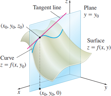
Similarly, Figure 31 shows that \(f_{y}( x_{0},y)\) is the slope of the tangent line to the curve \(z=f( x_{0},y)\), the curve of intersection of the plane \(x=x_{0}\) and the surface \(z=f(x,y)\).


THEOREM Slope of a Tangent Line
The partial derivative \(f_{x}(x_{0},y_{0})\) equals the slope of the tangent line to the curve of intersection of the surface \(z=f(x,y)\) and the plane \(y=y_{0}\) at the point \((x_{0},y_{0},f(x_{0},y_{0}) )\) on the surface \(z=f(x,y)\).
The partial derivative \(f_{y}(x_{0},y_{0})\) equals the slope of the tangent line to the curve of intersection of the surface \(z=f(x,y)\) and the plane \(x=x_{0}\) at the point \((x_{0},y_{0},f(x_{0},y_{0}) )\) on the surface \(z=f(x,y)\).
EXAMPLE 3Finding an Equation of a Tangent Line
NEED TO REVIEW?
Symmetric equations of a line in space are discussed in Section 10.6, pp. 734-735.
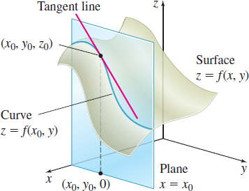
Find an equation of the tangent line to the curve of intersection of the surface \(z=f(x,y)=16-x^{2}-y^{2}\):
- (a) With the plane \(y=2\) at the point \((1,2,11)\)
- (b) With the plane \(x=1\) at the point \((1,2,11)\)
Solution (a) The slope of the tangent line to the curve of intersection of \(z=16-x^{2}-y^{2}\) and the plane \(y=2\) at any point is \( f_{x}(x,2)=-2x\). At the point \((1,2,11)\), the slope is \(f_{x}( 1,2) =-2(1) =\) \(-2\). This tangent line lies on the plane \( y=2\). Symmetric equations of the tangent line are \[ z-11= \frac{x-1}{-1/2}\qquad y=2 \]
(b) The slope of the tangent line to the curve of intersection of \(z=16-x^{2}-y^{2}\) and the plane \(x=1\) at any point is \(f_{y}(1,y)=-2y\). At the point \((1,2,11)\), the slope is \(f_{y}( 1,2) =-2( 2) =-4\). This tangent line lies on the plane \(x=1\). Symmetric equations of the tangent line are \[ z-11= \frac{y-2}{-1/4}\qquad x=1 \]
832
Figure 32 illustrates these solutions.
NOW WORK
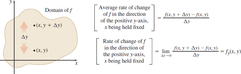
3 Interpret Partial Derivatives as a Rate of ChangePrinted Page 832
The definition of the partial derivatives of \(z=f(x,y)\) is a generalization of the definition of the derivative of a function of one variable. It is not surprising, therefore, to see similarities in the interpretations. For example, \(f_{x}(x,y)\) equals the rate of change of \(f\) in the direction of the positive \(x\)-axis (while \(y\) is held fixed), as shown in Figure 33.
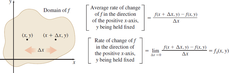
Similarly, \(f_{y}(x, y)\) equals the rate of change of \(f\) in the direction of the positive \(y\)-axis (\(x\) is held fixed), as shown in Figure 34.
NOTE
In Chapter 13, we discuss rates of change in any direction.
EXAMPLE 4Finding the Rate of Change of Temperature
The temperature \(T\) (in degrees Celsius) of a metal plate, located in the xy-plane, at any point \((x,y)\) is given by \(T=T(x,y) =24(x^{2}+y^{2})^{2}\).
- (a) Find the rate of change of \(T\) in the direction of the positive \(x\)-axis at the point \((1,-2)\).
- (b) Find the rate of change of \(T\) in the direction of the positive \(y\)-axis at the point \((1,-2)\).
Solution (a) The rate of change of temperature in the direction of the positive \(x\)-axis is given by \[ \begin{equation*} T_{x}(x, y)=2(24)(x^{2}+y^{2})(2x)=96\;x(x^2+y^2) \end{equation*} \]
833
At the point \((1,-2)\), \(T_{x}(1,-2)=96(1)(5) = 480\). This means that as one moves in a horizontal direction to the right away from the point \((1,-2)\), the temperature of the plate increases at the rate of \(480 ^\circ{\rm C}\) per unit of distance.
(b) The rate of change of temperature in the direction of the positive \(y\)-axis is given by \[ \begin{equation*} T_{y}(x, y)=2(24)(x^{2}+y^{2})(2y)=96\;y(x^2+y^2) \end{equation*} \]
At the point \((1,-2)\), \(T_{y}(1,-2)=96(-2) (5) =-960\). This means that as one moves in a vertical direction up from the point \((1,-2)\), the temperature of the plate decreases at the rate of \(960 {^\circ{\rm C}}\) per unit of distance.
NOW WORK
EXAMPLE 5Finding Rates of Change
See Figure 35.
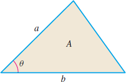
The area \(A\) of a triangle with sides \(a\) and \(b\) and included angle \(\theta \) is given by \[ A=\dfrac{1}{2}ab\;\sin\;\theta \]
- (a) Find the rate of change of \(A\) with respect to \(a\) when \(b\) and \(\theta\) are held fixed.
- (b) Find the rate of change of \(A\) with respect to \(b\) when \(a\) and \(\theta\) are held fixed.
- (c) Find the rate of change of \(A\) with respect to \(\theta\) when \(a\) and \(b\) are held fixed.
- (d) Evaluate each of the above if \(a=20\), \(b=30\), and \(\theta =\dfrac{\pi }{6}\).
- (e) Interpret the results found in (d).
Solution (a) \(\dfrac{\partial A}{\partial a}=\dfrac{1}{2}b\;\sin \theta\) (b) \(\dfrac{\partial A}{\partial b}=\dfrac{1}{2} a\;\sin \theta\) (c) \(\dfrac{\partial A}{\partial \theta }=\dfrac{1}{2}ab\;\cos \theta\) (d) When \(a=20\), \(b=30\), and \(\theta =\dfrac{\pi }{6}\), then \[ \begin{eqnarray*} \dfrac{\partial A}{\partial a} &=&\dfrac{1}{2}(30)\;\left( \sin \frac{\pi }{6}\right) =\dfrac{15}{2} \\[4pt] \dfrac{\partial A}{\partial b} &=&\dfrac{1}{2}(20)\;\left( \sin \frac{\pi }{6}\right) =5 \\[4pt] \dfrac{\partial A}{\partial \theta } &=&\dfrac{1}{2}\left( 20\right) (30)\;\cos \dfrac{\pi }{6}=150\sqrt{3} \end{eqnarray*} \]
(e) Each partial derivative equals the rate of change of area with respect to \(a,\) \(b,\) or \(\theta\). The relative size of each rate of change tells us that the area will increase most rapidly when \(a\) and \(b\) are fixed and \(\theta\) varies. The area increases the least when \(a\) and \(\theta\) are fixed and \(b\) varies.
In business and economics, analysts are often interested in the rate of change of a process, called the marginal process. For example, if the amount \(z\) of a good produced depends on the quantities of the \(x\) and \(y\) components used, then the production function \(z=f(x,y)\) gives the amount of output for the amounts \(x\) and \(y\) of input used. The marginal productivity of \(z\) with respect to an input \(x\) is \(f_{x}\) and the marginal productivity of \(z\) with respect to an input \(y\) is \(f_{y}\).
ORIGINS
Charles Wiggins Cobb (1875-1949) and Paul H. Douglas (1892-1976) were American scholars who studied the growth of the U.S. economy from 1899 to 1922. They produced a simple model, known as the Cobb–Douglas model, in which production output is a function of the amount of labor used and the amount of capital invested. Later, while Cobb continued to publish in mathematics (he obtained a PhD from the University of Michigan) and in economics, Douglas went into politics and represented Illinois in the U.S. Senate from 1949 to 1966.
EXAMPLE 6Finding Marginal Productivity: The Cobb–Douglas Model
In 1928 the mathematician Charles Cobb and the economist Paul Douglas empirically (from data) derived a production model for the manufacturing sector of the U.S. economy for the period 1899–1922. Using the model \(P=aK^{b}L^{1-b},\) where \(P\) is manufacturing productivity, \(K\) is capital input, and \(L\) is labor input, and multiple regression techniques, Cobb and Douglas determined that manufacturing productivity was represented by the function \[ P=1.014651K^{0.254124}L^{0.745876}\approx 1.01K^{0.25}L^{0.75} \]
834
- (a) Find the marginal productivity of manufacturing output with respect to capital input. Interpret the result.
- (b) Find the marginal productivity of manufacturing output with respect to labor input. Interpret the result.
Solution (a) The marginal productivity of manufacturing output with respect to capital input \(K\) is \[ \dfrac{\partial P}{\partial K}\approx 1.01( 0.25K^{-0.75}) L^{0.75}=0.2525\left( \dfrac{L}{K}\right) ^{0.75} \]
For every unit increase in capital input, there is an increase of \( 0.2525\left( \dfrac{L}{K}\right) ^{0.75}\) units in manufacturing productivity.
(b) The marginal productivity of manufacturing output with respect to labor input \(L\) is \[ \dfrac{\partial P}{\partial L}\approx 1.01K^{0.25}\left( 0.75L^{-0.25}\right) =0.7575\left( \dfrac{K}{L}\right) ^{0.25} \]
For every unit increase in labor input, there is an increase of \( 0.7575\left(\dfrac{K}{L}\right)^{0.25}\) units in manufacturing productivity.
Marginal productivity is usually positive. That is, as the amount of one input increases (with the other input held constant), the output also increases. However, as the input of one component increases, the output usually increases at a decreasing rate until the point is reached where there is no further increase in output. This is called the law of eventually diminishing marginal productivity.
NOW WORK
4 Find Second-Order Partial DerivativesPrinted Page 834
If the first-order partial derivatives of a function \(z=f(x,y)\) of two variables exist, and if it is possible to differentiate each of these with respect to \(x\) or \(y\), the result is four second-order partial derivatives. They are \[\bbox[5px, border:1px solid black, #F9F7ED]{\bbox[#FAF8ED,5pt]{ \begin{array}{lll} f_{xx}(x,y)=\dfrac{\partial }{\partial x}f_{x}(x,y)=\dfrac{\partial }{ \partial x}\dfrac{\partial z}{\partial x}=\dfrac{\partial ^{2}z}{\partial x^{2}}\qquad & f_{xy}(x,y)=\dfrac{\partial }{ \partial y}f_{x}(x,y)=\dfrac{\partial }{\partial y}\dfrac{\partial z}{ \partial x}=\dfrac{\partial ^{2}z}{\partial y\partial x} \\ f_{yx}(x,y)=\dfrac{\partial }{\partial x}f_{y}(x,y)=\dfrac{\partial }{ \partial x}\dfrac{\partial z}{\partial y}=\dfrac{\partial ^{2}z}{\partial x\,\partial y} & f_{yy}(x,y)=\dfrac{\partial }{\partial y}f_{y}(x,y)= \dfrac{\partial }{\partial y}\dfrac{\partial z}{\partial y}=\dfrac{\partial ^{2}z}{\partial y^{2}} \end{array}}} \]
The two second-order partial derivatives \[ \begin{equation*} \frac{\partial ^{2}z}{\partial x\partial y}=f_{yx}(x, y)\qquad \hbox{and} \qquad \frac{\partial ^{2}z}{\partial y\partial x}=f_{xy}(x, y) \end{equation*} \]
are called mixed partials.
CAUTION
Notice the differences in the two mixed partial derivatives. To find \(\dfrac{\partial^{2}z}{\partial x\partial y}=f_{yx}\), first differentiate \(f\) with respect to \(y\) and then differentiate \(f_{y}\) with respect to \(x,\) in that order. On the other hand, to find \(\dfrac{\partial ^{2}z}{\partial y\partial x}=f_{xy}\), first differentiate \(f\) with respect to \(x\) and then differentiate \(f_{x}\) with respect to \(y\).
835
EXAMPLE 7Finding Second-Order Partial Derivatives
Find the four second-order partial derivatives of \(z=f(x,y)=x\;\ln\;y+ye^{x}\).
Solution We begin by finding the first-order partial derivatives \(f_{x}(x,y)\) and \(f_{y}(x,y)\). \[ f_{x}(x,y)=\ln\;y+ye^{x} \qquad f_{y}(x,y)=\dfrac{x}{y}+e^{x} \]
Then the second-order partial derivatives are \[ \begin{array}{lll} f_{xx}(x,y)&=&\dfrac{\partial }{\partial x}f_{x}(x,y)=\dfrac{\partial }{\partial x}\left(\ln\;y+ye^{x}\right) =ye^{x} & f_{xy}(x,y)&=&\dfrac{\partial }{\partial y}f_{x}(x,y)=\dfrac{\partial }{\partial y}\left(\ln\;y+ye^{x}\right) =\dfrac{1}{y}+e^{x} \\[5pt] f_{yx}(x,y)&=&\dfrac{\partial }{\partial x}f_{y}(x,y)=\dfrac{\partial }{\partial x}\left(\dfrac{x}{y}+e^{x}\right) =\dfrac{1}{y}+e^{x} & \quad f_{yy}(x,y)&=&\dfrac{\partial }{\partial y}f_{y}(x,y)=\dfrac{\partial }{\partial y}\left( \dfrac{x}{y}+e^{x}\right) =-\dfrac{x}{y^{2}} \end{array} \]
Notice in Example 7 that the mixed partials \(f_{xy}\) and \( f_{yx}\) are equal. As it turns out, the mixed partials are equal for most functions we encounter. The next result gives conditions for the mixed partials to be equal.
NOW WORK
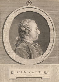
THEOREM Equality of Mixed Partials (Clairaut’s Theorem)
Let \(z=f(x,y)\) be a function of two variables whose domain is the set \(D\). Let \((x_{0},y_{0})\) be an interior point of \(D\). If the partial derivatives \(f_{x}\), \(f_{y}\), \(f_{xy}\), and \(f_{yx}\) exist at each point of some disk centered at \((x_{0},y_{0})\), and if \(f_{xy}\) and \( f_{yx}\) are continuous at \((x_{0},y_{0})\), then \(f_{x y}(x_{0},y_{0})=f_{yx}(x_{0},y_{0})\).
ORIGINS
Alexis Claude Clairaut (1713–1765) was home schooled by his father, a respected mathematician. As a result, Clairaut completed algebra when he was 9, produced his first scholarly paper at age 13, and was the youngest person admitted to the Paris Academy of Sciences. When he was about 30, Clairaut began to study the three-body problem–seeking a solution to the motion of three masses that attract each other according to Newton’s Law. He applied this theory to the orbit of Halley’s comet, and was able to predict the return of the comet to within weeks.
A proof of Clairaut’s Theorem may be found in most advanced calculus texts. For an example of a function for which the mixed partials are not equal, see Problem 75 or 76.
Continuity and Partial Derivatives
In Chapter 2, we proved the important result that if a function \(f\) of one variable has a derivative at \(c\), then \(f\) is continuous at \(c\). This property is not necessarily true for a function \(f\) of several variables. That is, if a function \(f\) of several variables has partial derivatives at a point \(P_{0}\), the function \(f\) may fail to be continuous at \(P_{0}\).
EXAMPLE 8Showing That a Function of Two Variables Having Partial Derivatives Is Not Continuous
Show that the function \[ f(x, y)=\left\{ \begin{array}{@{}c@{\quad}c@{\quad}c} \dfrac{xy}{x^{2}+y^{2}} & \hbox{if} & (x,y)\neq (0,0) \\ 0 & \hbox{if} & (x,y)=(0,0) \end{array} \right. \]
has partial derivatives at \((0,0),\) but is not continuous at that point.
836
Solution We use the definition to find the partial derivatives of \(f\) at \((0,0)\). 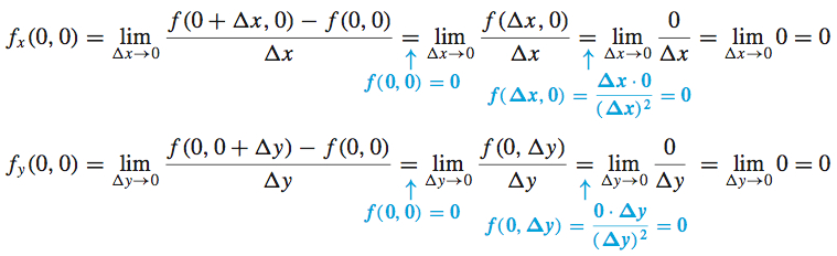
The partial derivatives \(f_{x}(0,0)\) and \(f_{y}(0,0)\) both exist.
But \(\lim\limits_{(x, y)\rightarrow (0, 0)}\dfrac{xy}{x^{2}+y^{2}}\) does not exist. (See Example 2 from Section 12.2.) As a result, \(f\) is not continuous at \((0,0)\).
NOW WORK
5 Find the Partial Derivatives of a Function of \(n\) VariablesPrinted Page 836
The idea of partial differentiation can be extended to functions of three or more variables. If \(w=f(x,y,z)\) is a function of three variables, there will be three first-order partial derivatives:
- The partial derivative of \(w\) with respect to \(x\) is \(\dfrac{\partial w}{ \partial x}=f_{x}(x,y,z)\).
- The partial derivative of \(w\) with respect to \(y\) is \(\dfrac{\partial w}{ \partial y}=f_{y}(x,y,z)\).
- The partial derivative of \(w\) with respect to \(z\) is \(\dfrac{\partial w}{ \partial z}=\) \(f_{z}(x,y,z)\).
Each partial derivative is found by differentiating with respect to the indicated variable, while treating the other two variables as constants.
The function \(f_{x}\) equals the rate of change of \(w\) with respect to \(x\); the function \(f_{y}\) equals the rate of change of \(w\) with respect to \(y\); and the function \(f_{z}\) equals the rate of change of \(w\) with respect to \(z\).
EXAMPLE 9Finding the Partial Derivatives of a Function of Three Variables
If \(w=f(x,y,z)=5x^{2}yz^{3}\), then \[ f_{x}(x,y,z)=10xyz^{3}\qquad f_{y}(x,y,z)=5x^{2}z^{3}\qquad f_{z}(x,y,z)=15x^{2}yz^{2} \]
NOW WORK
Higher-order partial derivatives of a function \(w=f(x,y,z)\) of three variables are defined in a similar way to those of a function of two variables. For example, \[ f_{zy}=\frac{\partial }{\partial y}\left( \frac{\partial w}{\partial z} \right) =\frac{\partial ^{2}w}{\partial y\partial z}\qquad \hbox{and}\qquad f_{xz}=\frac{\partial }{\partial z}\left( \frac{\partial w}{ \partial x}\right) =\frac{\partial ^{2}w}{\partial z\partial x} \]
837
As in the case of functions of two variables, for most functions \(w=f(x,y,z)\) , the mixed partials have the property that \(f_{xy}=f_{yx}\) and \( f_{xz}=f_{zx}\) and \(f_{yz}=f_{zy}\).
If \(z=f(x_{1}, x_{2}, \ldots , x_{n})\) is a function of \(n\) variables, there are \(n\) partial derivatives of \(f\). The partial derivative of \(f\) with respect to \(x_{1}, \dfrac{\partial f}{\partial x_{1}}\), is found by differentiating \(f\) with respect to \(x_{1}\), while treating the remaining variables as constants. The other partial derivatives \(\dfrac{\partial f}{ \partial x_{2}}, \dfrac{\partial f}{\partial x_{3}}, \ldots , \dfrac{ \partial f}{\partial x_{n}}\) are defined similarly.
EXAMPLE 10Finding the Partial Derivatives of a Function of \(n\) Variables
If \(z=f(x_{1}, x_{2}, \ldots , x_{n})=x_{1}^{2}+x_{2}^{2}+\cdots +x_{n}^{2}\), then \[ \frac{\partial f}{\partial x_{1}}=2x_{1} \qquad \frac{\partial f}{\partial x_{2}}=2x_{2}\qquad \ldots \qquad \frac{\partial f}{\partial x_{n}}=2x_{n} \]
Collectively, these partial derivatives can be written as \[ \frac{\partial f}{\partial x_{i}}=2x_{i} \qquad \hbox{where } i=1,2, \ldots , n \]