13 Inference in Regression

Section 13.3 Exercises

CLARIFYING THE CONCEPTS

Question 13.103

1. Write the multiple regression equation for $k = 3$ predictor variables. (p. 743)

13.3.1

$\hat{y} = b_{0} + b_{1} x_{1} + b_{2} x_{2} + b_{3} x_{3}$

Question 13.104

2. Which is preferable, $R^{2}$ or $R_{adj}^{2}$ , and why? (p. 745)

Question 13.105

3. Which test do we perform if we want to determine whether our multiple regression is useful? (p. 746)

13.3.3

The $F$ test for the overall significance of the multiple regression

Question 13.106

4. If we conclude from the $F$ test thatour multiple regression is useful, is it still possible that one of the $β^{,}$ s equals zero? Explain. (p. 746)

Question 13.107

5. Explain the difference between the $F$ test and the $t$ test we learned in this section. (p. 747)

13.3.5

The $F$ test is for the overall significance of the multiple regression and the $t$ test is for testing whether a particular $x$ -variable has a significant relationship with the response variable $y$ .

Question 13.108

6. How many $t$ tests may we perform for a multiple regression model? (p. 747)

Question 13.109

7. How do we interpret the coefficient for a dummy variable. (Hint: Consider Figure 29.) (p. 750)

13.3.7

The coefficient of a dummy variable can be interpreted as the estimated increase in $y$ for those observations with the value of the dummy variable equal to 1 as compared to those with the value of the dummy variable equal to 0 when all of the other $x$ variables are held constant.

Question 13.110

8. What are the four steps of the Strategy for Building a Multiple Regression Model. (p. 750)

PRACTICING THE TECHNIQUES

CHECK IT OUT!

To do	Check out	Topic
Exercises 9–16	Example 11	Multiple regression equation, coefficients, and predictions
Exercises 17–20	Example 12	Calculating and interpreting the adjusted coefficient of determination $R_{adj}^{2}$
Exercises 21–22 and 27–28	Example 13	$F$ test for the overall significance of the multiple regression
Exercises 23 and 30	Example 14	Performing a set of $t$ tests for the significance of a set of individual $x$ variables
Exercise 29	Example 15	Dummy variables in multiple regression
Exercises 24–26 and 31–33	Example 16	Strategy for building a multiple regression model

Use the following information for Exercises 9–12: A multiple regression model has been produced for a set of $n = 20$ observations with multiple regression equation $\hat{y} = 10 + 5 x_{1} + 8 x_{2}$ , with multiple coefficient of determination $R^{2} = 0.5$ .

Assume the regression assumptions are met.

Question 13.111

9. Interpret the value of the coefficient for $x_{1}$ .

13.3.9

For each increase in one unit of the variable $x_{1}$ , the estimated value of $y$ increases by 5 units when the value of $x_{2}$ is held constant.

Question 13.112

10. Explain what the value of $b_{2}$ means.

Question 13.113

11. Interpret the coefficients $b_{0}, b_{1},$ , and $b_{2}$ .

13.3.11

The estimated value of $y$ when $x_{1} = 0$ and $x_{2} = 0$ is $b_{0} = 10$ . $b_{1} = 5$ means that for each increase of one unit of the variable $x_{1}$ , the estimated value of $y$ increases by 5 units when the value of $x_{2}$ is held constant. $b_{2} = 8$ means that for each increase of one unit of the variable $x_{2}$ , the estimated value of $y$ increases by 8 units when the value of $x_{1}$ is held constant.

Question 13.114

12. Find point estimates of $y$ for the following values of $x_{1}$ and $x_{2}$ :

$x_{1} = 6, x_{2} = 4$
$x_{1} = 10, x_{2} = 8$

Use the following information for Exercises 13–16: A multiple regression model has been produced for a set of $n = 50$ observations with multiple regression equation $\hat{y} = 0.5 - 0.1 x_{1} + 0.9 x_{2}$ , with multiple coefficient of determination $R^{2} = 0.75$ . Assume the regression assumptions are met.

Question 13.115

13. Interpret the value of the coefficient for $x_{1}$ .

13.3.13

For each increase in one unit of the variable $x_{1}$ , the estimated value of $y$ decreases by 0.1 unit when the value of $x_{2}$ is held constant.

Question 13.116

14. Explain what the value of $b_{2}$ means.

Question 13.117

15. Interpret the coefficients $b_{0}, b_{1}$ , and $b_{2}$ .

13.3.15

The estimated value of $y$ when $x_{1} = 0$ and $x_{2} = 0$ is $b_{0} = 0.5$ . $b_{1} = - 0.1$ means that for each increase of one unit of the variable $x_{1}$ , the estimated value of $y$ decreases by 0.1 unit when the value of $x_{2}$ is held constant. $b_{2} = 0.9$ means that for each increase of one unit of the variable $x_{2}$ , the estimated value of $y$ increases by 0.9 unit when the value of $x_{1}$ is held constant.

Question 13.118

16. Find point estimates of $y$ for the following values of $x_{1}$ and $x_{2}$ :

$x_{1} = 5, x_{2} = 6$
$x_{1} = 4, x_{2} = 3$

Question 13.119

17. For the data in Exercises 9–12, how should the value of $R^{2}$ be interpreted?

13.3.17

50% of the variability in $y$ is accounted for by this multiple regression equation.

Question 13.120

18. Calculate $R_{adj}^{2}$ for the data in Exercises 9–12.

Question 13.121

19. For the data in Exercises 13–16, how should the value of $R^{2}$ be interpreted?

13.3.19

75% of the variability in $y$ is accounted for by this multiple regression equation.

Question 13.122

20. Calculate $R_{adj}^{2}$ for the data in Exercises 13–16.

Page 755

Use the following data set for Exercises 21-26.

$y$	$x_{1}$	$x_{2}$	$x_{3}$
0.6	1	10	1.3
4.0	2	10	−3.2
3.2	3	8	−1.0
9.0	4	8	0.9
1.8	5	6	−2.5
8.4	6	6	0.9
9.8	7	4	1.0
10.4	8	4	2.0
8.8	9	2	0.2
14.7	10	2	−2.2

Question 13.123

21. Perform the multiple regression of $y$ on $x_{1}$ , $x_{2}$ , and $x_{3}$ , and write the multiple regression equation.

13.3.21

$\hat{y} = - 37.8 + 4.50 x_{1} + 3.37 x_{2} + 0.306 x_{3}$

Question 13.124

22. Assume the regression assumptions are met. Perform the $F$ test for the significance of the overall regression, using level of significance $α = 0.05$ . Do the following:

State the hypotheses and the rejection rule.
Find the $F$ statistic and the $p$ value.
State the conclusion and interpretation.

Question 13.125

23. Perform the $t$ test for the significance of the individual predictor variables, using level of significance $α = 0.05$ . Do the following:

For each hypothesis test, state the hypotheses and the rejection rule.
For each hypothesis test, find the $t$ statistic and the $p$ -value.
For each hypothesis test, state the conclusion and interpretation.

13.3.23

(a) Test $H_{0} : β_{1}$ : There is no linear relationship between $y$ and $x_{1}$ . $H_{a} : β_{1}$ : There is a linear relationship between $y$ and $x_{1}$ . Reject $H_{0}$ if the $p$ -value $\leq α = 0.05$ . Test 2: $H_{0} : β_{2}$ : There is no linear relationship between $y$ and $x_{2}$ . $H_{a} : β_{2}$ : There is a linear relationship between $y$ and $x_{2}$ . Reject $H_{0}$ if the $p$ -value $\leq α = 0.05$ . Test 3: $H_{0} : β_{3} = 0$ : There is no linear relationship between $y$ and $x_{3}$ . $H_{a} : β_{3} \neq 0$ : There is a linear relationship between $y$ and $x_{3}$ . Reject $H_{0}$ if the $p$ -value $\leq α = 0.05$ . (b) Test $1 : t = 3.72$ , with $p -value = 0.010$ . Test $2 : t = 2.75$ , with $p -value = 0.034$ . Test $3 : t = 0.87$ , with $p -value = 0.418$ . (c) Test 1: The $p -value = 0.010$ , which is $\leq α = 0.05$ . Therefore we reject $H_{0}$ . There is evidence of a linear relationship between $y$ and $x_{1}$ . Test 2: The $p -value = 0.034$ , which is $\leq α = 0.05$ . Therefore we reject $H_{0}$ . There is evidence of a linear relationship between $y$ and $x_{2}$ . Test 3: The $p -value = 0.418$ , which is not $\leq α = 0.05$ . Therefore we do not reject $H_{0}$ . There is insufficient evidence of a linear relationship between $y$ and $x_{3}$ .

Question 13.126

24. Identify any predictors that have corresponding $p$ -values greater than the level of significance $α = 0.05$ . Of these, discard the variable with the largest $p$ -value. Then redo Exercise 23, omitting this predictor. Repeat if necessary.

Question 13.127

25. Verify the regression assumptions for your final model from Exercise 24.

13.3.25

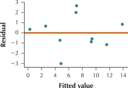
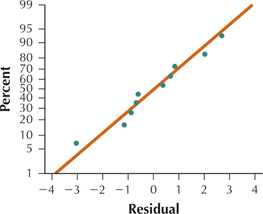
The scatterplot above of the residuals versus fitted values shows no strong evidence of unhealthy patterns. Thus, the independence assumption, the constant variance assumption, and the zero-mean assumption are verified. Also, the normal probability plot of the residuals above indicates no evidence of departure from normality of the residuals. Therefore we conclude that the regression assumptions are verified.

Question 13.128

26. Report and interpret your final model from Exercise 24, by doing the following:

Provide the multiple regression equation for your final model.
Interpret the multiple regression coefficients so that a nonstatistician could understand.
Report and interpret the standard error of the estimate $s$ and the adjusted coefficient of determination $R_{adj}^{2}$ .

Use the following data set for Exercises 27–33. Note that $x_{3}$ is a dummy variable.

$y$	$x_{1}$	$x_{2}$	$x_{3}$
−0.7	2	0.1	0
6.4	4	−2.5	1
2.8	6	2.7	0
9.4	8	2.8	1
8.6	10	−1.6	0
13.1	12	1.0	1
12.2	14	−1.4	0
19.1	16	−0.5	1
18.8	18	1.0	0
23.2	20	−2.3	1

Question 13.129

27. Perform the multiple regression of $y$ on $x_{1}$ , $x_{2}$ , and $x_{3}$ , and write the multiple regression equation.

13.3.27

The regression equation is $\hat{y} = - 2.98 + 1.13 x_{1} - 0.175 x_{2} + 3.55 x_{3}$ .

Question 13.130

28. Assume the regression assumptions are met. Perform the $F$ test for the significance of the overall regression, using level of significance $α = 0.01$ . Do the following:

State the hypotheses and the rejection rule.
Find the $F$ statistic and the $p$ -value.
State the conclusion and interpretation.

Question 13.131

29. Interpret the coefficient for the dummy variable.

13.3.29

For each increase in one unit of the variable $x_{3}$ , the estimated value of $y$ increases by 3.55 units when the values of $x_{1}$ and $x_{2}$ are held constant.

Question 13.132

30. Perform the $t$ test for the significance of the individual predictor variables, using level of significance $α = 0.01$ . Do the following:

For each hypothesis test, state the hypotheses and the rejection rule.
For each hypothesis test, find the $t$ statistic and the $p$ -value.
For each hypothesis test, state the conclusion and interpretation.

Question 13.133

31. Identify any predictors that have corresponding $p$ -values greater than the level of significance $α = 0.01$ . Of these, discard the variable with the largest $p$ -value. Then redo Exercise 30, omitting this predictor. Repeat if necessary.

13.3.31

The $p$ -value for $x_{2}$ is the only $p$ -value greater than $α = 0.01$ , so we eliminate $x_{2}$ from the multiple regression equation. The new regression equation is $\hat{y} = - 3.12 + 1.15 x_{1} + 3.61 x_{3}$ . (a) Test $1 : H_{0} : β_{1} = 0$ : There is no linear relationship between $y$ and $x_{1}$ . $H_{a} : β_{1} \neq 0$ : There is a linear relationship between $y$ and $x_{1}$ . Reject $H_{0}$ if the $p$ -value $\leq α = 0.01$ . Test $2 : H_{0} : β_{3} = 0$ There is no linear relationship between $y$ and $x_{3}$ . $H_{a} : β_{3} \neq 0$ : There is a linear relationship between $y$ and $x_{3}$ . Reject $H_{0}$ if the $p$ -value $\leq α = 0.01$ . (b) Test 1: $t = 21.38$ , with $p -value = 0.000$ ; Test 2: $t = 5.86$ , with $p -value = 0.001$ . (c) Test 1: The $p -value = 0.000$ , which is $\leq α = 0.01$ . Therefore we reject $H_{0}$ . There is evidence of a linear relationship between $y$ and $x_{1}$ . Test 2: The $p -value = 0.001$ , which is $\leq α = 0.01$ . Therefore we reject $H_{0}$ . There is evidence of a linear relationship between $y$ and $x_{3}$ . Since all of the variables are significant, we have our final multiple regression equation.

Question 13.134

32. Verify the regression assumptions for your final model from Exercise 31.

Question 13.135

33. Report and interpret your final model from Exercise 31, by doing the following:

Provide the multiple regression equation for your final model.
Interpret the multiple regression coefficients so that a nonstatistician could understand.
Report and interpret the standard error of the estimate $s$ , and the adjusted coefficient of determination $R_{adj}^{2}$ .

13.3.33

(a) The final multiple regression equation is $\hat{y} = - 3.12 + 1.15 x_{1} + 3.61 x_{3}$ . For $x_{3} = 0$ , the regression equation is $\hat{y} = - 3.12 + 1.15 x_{1}$ . For $x_{3} = 1$ , the regression equation is $\hat{y} = 0.49 + 1.15 x_{1}$ . (b) For each increase in one unit of the variable $x_{1}$ , the estimated value of $y$ increases by 1.15 units. The estimated increase in $y$ for those observations with $x_{3} = 1$ , as compared to those with $x_{3} = 0$ , when $x_{1}$ is held constant, is 3.61. (c) Using the multiple regression equation in (a), the size of the typical prediction error will be about 0.959129. 98.4% of the variability in $y$ is accounted for by this multiple regression equation.

APPLYING THE CONCEPTS

For Exercises 34–39, apply the Strategy for Building a Multiple Regression Model by performing the following steps, using level of significance $α = 0.05$ :

Step 1 Perform the $F$ test for significance of the overall regression.
Step 2 Perform the $t$ tests for the individual predictors. If at least one of the predictors is not significant, then eliminate the $x$ variable with the largest $p$ -value from the model. Repeat Step 2 until all remaining predictors are significant.
Step 3 Verify the assumptions.
Step 4 Report and interpret your final model. Report and interpret the coefficients, the standard error of the estimate $s$ , and the adjusted coefficient of determination $R_{adj}^{2}$ .

Question 13.136

bestdating

34. Best Places for Dating. Sperling's Best Places published the list of best places for dating in America for 2010. Table 6 shows the top 10 places, along with the overall dating score ( $y$ ) and a set of predictor variables.

Page 756

Table 13.42: TABLE 6 Best places for dating in America

City	$y$ = Overall dating score	Percentage 18–24 years old	Percentage 18–24 years and single	Online dating score
Austin	100.0	13.40%	81.20%	77.8
Colorado Springs	88.7	10.50%	74.20%	88.9
San Diego	84.0	11.30%	79.40%	77.4
Raleigh	80.7	11.60%	82.90%	79.2
Seattle	78.7	9.00%	83.90%	100.0
Charleston	78.7	11.20%	82.70%	66.9
Norfolk	77.0	11.20%	75.60%	82.9
Ann Arbor	75.5	12.90%	90.30%	51.1
Springfield	75.2	11.70%	89.80%	63.5
Honolulu	75.2	10.10%	82.30%	50.2

Question 13.137

bestbusiness

35. Ease of Doing Business. Doing Business (www.doingbusiness.org) publishes statistics on how easy or difficult different countries make it to do business. Table 7 shows the top 12 countries for ease of doing business, with $y = easiness score along with a set of predictor variables$ .

Table 13.43: TABLE 7 Best countries for ease of doing business

Country	Easiness score	Starting a business	Employing workers	Paying taxes
Singapore	100	10	1	5
New Zealand	99	1	14	12
United States	98	6	1	46
Hong Kong	97	15	20	3
Denmark	96	16	10	13
U.K.	95	8	28	16
Ireland	94	5	38	6
Canada	93	2	18	28
Australia	92	3	8	48
Norway	91	33	99	18
Iceland	90	17	62	32
Japan	89	64	17	112

13.3.35

See Solutions Manual.

Question 13.138

vaweather

36. Virginia Weather. Table 8 contains data on weather in a sample of cities in the state of Virginia. We are interested in predicting $y = heating degree days using the other predictor variables$ .

Table 13.44: TABLE 8 Data on the weather in Virginia

City	Heating degreedays	Avg. Jan. temp.	Avg. July temp.	Cooling degreedays
Alexandria	4055	34.9	79.2	1531
Arlington	4055	34.9	79.2	1531
Blacksburg	5559	30.9	71.1	533
Charlottesville	4103	35.5	76.9	1212
Chesapeake	3368	40.1	79.1	1612
Danville	3970	36.6	78.8	1418
Hampton	3535	39.4	78.5	1432
Harrisonburg	5333	30.5	73.5	758
Leesburg	5031	31.5	75.2	911
Lynchburg	4354	34.5	75.1	1075
Manassas	4925	31.7	75.7	1075
Newport News	3179	41.2	80.3	1682
Norfolk	3368	40.1	79.1	1612
Petersburg	3334	39.7	79.6	1619
Portsmouth	3368	40.1	79.1	1612
Richmond	3919	36.4	77.9	1435
Roanoke	4284	35.8	76.2	1134
Suffolk	3467	39.6	78.5	1427
Virginia Beach	3336	40.7	78.8	1482

Table 13.44: Source: National Oceanic and Atmospheric Administration.

Question 13.139

healthinsurance

37. Health Insurance Coverage. We are interested in estimating $y = the number of people covered by health insurance$ , using $x_{1} = the number of adults not covered$ and $x_{2} = the number of children not covered$ . Use the data in Table 9, containing a random sample of U.S. states. All data are in thousands.

Table 13.45: TABLE 9 Health insurance coverage

State	Persons covered	Adults not covered	Children not covered
Alabama	3,843	689	82
Arizona	4,958	1,311	283
Colorado	3,977	826	176
Georgia	7,688	1,659	314
Illinois	10,867	1,776	302
Kentucky	3,467	639	98
Maryland	4,836	776	137
Massachusetts	5,678	657	103
Michigan	8,928	1,043	116
Minnesota	4,675	475	104
Missouri	5,028	772	127
New Jersey	7,319	1,341	277
North Carolina	7,266	1,585	307
Ohio	10,181	1,138	157
Pennsylvania	11,108	1,237	203
South Carolina	3,553	672	112
Tennessee	5,111	809	94
Virginia	6,532	1,006	185
Washington	5,572	746	105
Wisconsin	4,995	481	63

13.3.37

See Solutions Manual.

Page 757

Question 13.140

accounting

38. Regression in Accounting. We are interested in estimating $y = current ratio$ using $x_{1} = price - earnings ratio$ , $x_{2} = total assets$ , and $x_{3} = total liabilities$ . Use the data in Table 10, containing a random sample of large technology companies in 2010. Total assets and total liabilities are in billions of dollars.

Table 13.46: TABLE 10 Accounting data for large technology companies

Company	Current ratio	Price–earnings ratio	Assets	Liabilities
Microsoft	1.82	12.51	77.9	38.3
Intel	2.79	18.44	53.1	11.4
Dell	1.28	10.95	33.7	28.0
Apple	1.88	24.57	53.9	26.0
Google	10.62	18.87	40.5	4.5

Table 13.46: Source: Lexis-Nexis.

Build the final multiple regression model using level of significance $α = 0.10$ .
Comment on your results from (a).
Redo your work from (a), this time using level of significance $α = 0.13$ .
Report and interpret your final model from (c).

Question 13.141

systolic

39. Blood Pressure. Open the data set Systolic. We are interested in estimating $y = systolic blood pressure$ , based on the other predictor variables.

13.3.39

See Solutions Manual.

Question 13.142

40. Baseball. In Example 16, interpret the coefficients for Triples, Hits, Home Runs, RBIs, Walks, and Red Sox.

Your Best Model. Work with the Nutrition data sets for Exercises 41 and 42.

Question 13.143

nutrition

41. Use technology to apply the Strategy for Building a Multiple Regression Model, using level of significance $α = 0.05$ , for predicting the number of calories, with the following $x$ -variables: protein, fat, saturated fat, cholesterol, carbohydrates, calcium, phosphorous, iron, potassium, sodium, thiamin, niacin, and ascorbic acid.

13.3.41

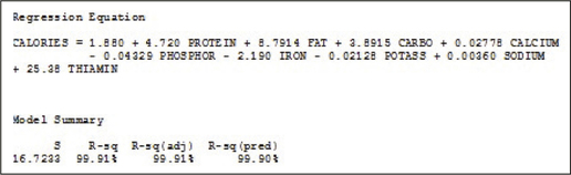
The standard error in the estimate for the final model is $s = 16.7233$ . That is, using the multiple regression equation given above, the size of the typical prediction error will be about 16.7233 calories. The adjusted coefficient of variation is $R_{adj}^{2} = 99.91 %$ . In other words, 99.91% of the variation in calories is accounted for by this multiple regression equation.

Question 13.144

nutrition

42. Write a summary to interpret each regression coefficient, and comment on which variables are the most important for predicting the number of calories.