Section 6.1Exercises
CLARIFYING THE CONCEPTS
Question 6.1
1. Explain in your own words what a random variable is. Give an example of a random variable from your own life experience. (p. 310)
6.1.1
Answers will vary.
Question 6.2
2. Is your height a random variable? Under what circumstances is your height considered a random variable? Under what circumstances is your height not considered a random variable? (p. 310)
Question 6.3
3. What is the difference between a discrete random variable and a continuous random variable? (p. 311)
6.1.3
Discrete: takes finite or a countable number of values that can be graphed as separate points on the number line; continuous takes infinitely many values that form an interval on the number line.
Question 6.4
4. What is the difference between a discrete random variable and a discrete probability distribution? (p. 312)
Question 6.5
5. What are the two rules for a discrete probability distribution? (p. 313)
6.1.5
ΣP(X)=1 and 0≤P(X)≤1.
Question 6.6
6. Explain the difference between from Section 3.1 and the mean of a discrete random variable. (p. 317)
PRACTICING THE TECHNIQUES
 CHECK IT OUT!
| To do | Check out | Topic |
|---|---|---|
| Exercises 7–16 |
Example 2 | Identifying discrete and continuous random variables (RVs) |
| Exercises 17a–24a |
Example 3 | Probability distribution table |
| Exercises 25–28 |
Example 4 | Recognizing valid discrete probability distributions |
| Exercises 17b–24b |
Example 5 | Discrete probability distribution as a graph |
| Exercises 29–44 |
Example 6 | Calculating probabilities for multiple values of |
| Exercises 45a–52a |
Example 7 | Calculating the mean of a discrete probability distribution |
| Exercises 45b–52b |
Example 9 | Identifying the most likely value of a discrete RV |
| Exercises 45c–52c |
Example 10 | Expected value of a discrete RV |
| Exercises 53a,b–60a,b |
Example 11 | Calculating the variance and standard deviation of a discrete RV |
| Exercises 53c–60c |
Example 12 |
-score method for determining an unusual value |
For Exercises 7–12, indicate whether the variable is a discrete or continuous random variable.
Question 6.7
7. The number of siblings that a randomly chosen person has
6.1.7
Discrete
Question 6.8
8. How long you will wait in your next checkout line
Question 6.9
9. How much coffee will be in your next cup of coffee
6.1.9
Continuous
Question 6.10
10. How hot it will be the next time you visit the beach
Question 6.11
11. The number of correct answers on your next multiple-choice quiz
6.1.11
Discrete
Question 6.12
12. How many songs you download this month
For Exercises 13–16, write down the possible values of the discrete random variables.
Question 6.13
13. The number of students in a classroom where the maximum class size is 15
6.1.13
{0, 1, 2, 3, 4, 5, 6, 7, 8, 9, 10, 11, 12, 13, 14, 15}
Question 6.14
14. How many different fingers on which you will get paper cuts next week
Question 6.15
15. The number of games that the California Angels will win the next time they are in the World Series (maximum = 4)
6.1.15
{0, 1, 2, 3, 4}
Question 6.16
16. The number of Donald Duck's three nephews, Huey, Dewey, and Louie, who will get into trouble in their next cartoon adventure
For Exercises 17–24, use the given information to do the following for the indicated random variable :
- Construct a probability distribution table.
- Construct a probability distribution graph.
Question 6.17
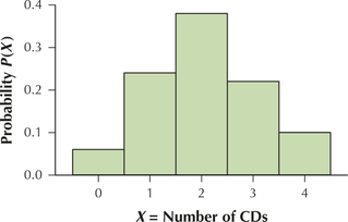
17. Shirelle enjoys listening to album downloads while doing her homework. The probabilities that she will listen to album downloads tonight are 6%, 24%, 38%, 22%, and 10%, respectively.
6.1.17
(a)
| 0 | 1 | 2 | 3 | 4 | |
| 0.06 | 0.24 | 0.38 | 0.22 | 0.10 |
(b)
Question 6.18
18. Josefina loves to score goals for her college soccer team. The probabilities that she will score goals tonight are 0.25, 0.35, 0.25, and 0.15, respectively.
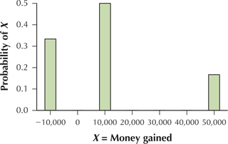
Question 6.19
19. Joshua is going to make it big on Wall Street, if only he can graduate from college first. Joshua has invested money in a high-risk mutual fund, and has figured his probability of losing $10,000 to be one-third, his probability of gaining $10,000 to be one-half, and his probability of gaining $50,000 to be one-sixth. Let .
6.1.19
(a)
| −$10,000 | $10,000 | $50,000 | |
| 1/3 | 1/2 | 1/6 |
(b)
Question 6.20
20. Chelsea is looking for a roommate, and would prefer one who had either one or two pets. Of the 10 possible roommates who answered Chelsea's ad, 5 have no pets, 3 have one pet, 1 has two pets, and 1 has three pets.
Question 6.21
stanleycup
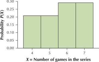
21. The National Hockey League championship is decided by a best-of-seven playoff called the Stanley Cup Finals. The following table shows the possible values of , and the frequency of each value of , for the Stanley Cup Finals between 1990 and 2014.
| Frequency | |
|---|---|
| 4 | 5 |
| 5 | 5 |
| 6 | 7 |
| 7 | 7 |
6.1.21
(a)
| 4 | 0.2083 |
| 5 | 0.2083 |
| 6 | 0.2917 |
| 7 | 0.2917 |
| Total | 1.0000 |
(b)
Question 6.22
22. The College Board reported for 2014 that, among students who took SAT subject tests, 29,000 students took one SAT subject test, 103,000 took two SAT subject tests, and 90,000 took three. (Hint: Find the sum. Then divide each number of students by the sum to get the probabilities.)
Question 6.23
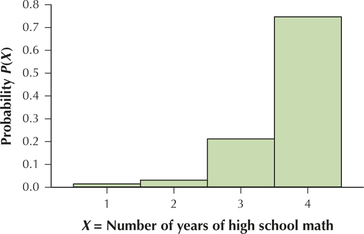
23. For 2014, the College Board reported that 742,000 students had 4 years of high school math, 209,000 had three years of high school math, 30,000 had two years, and 13,000 had one year of high school math when they took their SAT exams.
6.1.23
(a)
| 4 | 0.7465 |
| 3 | 0.2103 |
| 2 | 0.0302 |
| 1 | 0.0131 |
| Total | 1.0001 |
(b)
Question 6.24
hurricanes
24. The National Oceanic and Atmospheric Administration reports the following number of major hurricanes per year for the years 1989-2013.
| Year | Major hurricanes | Year | Major hurricanes |
|---|---|---|---|
| 1989 | 2 | 2002 | 2 |
| 1990 | 1 | 2003 | 3 |
| 1991 | 2 | 2004 | 6 |
| 1992 | 1 | 2005 | 7 |
| 1993 | 1 | 2006 | 2 |
| 1994 | 0 | 2007 | 2 |
| 1995 | 5 | 2008 | 5 |
| 1996 | 6 | 2009 | 2 |
| 1997 | 1 | 2010 | 5 |
| 1998 | 3 | 2011 | 4 |
| 1999 | 5 | 2012 | 2 |
| 2000 | 3 | 2013 | 0 |
| 2001 | 4 |
For Exercises 25–28, determine whether the distribution represents a valid probability distribution. If it does not, explain why not.
Question 6.25
25.
| −10 | 0 | 10 | |
|---|---|---|---|
| 1/5 | 1/2 | 1/5 |
6.1.25
Not a valid probability distribution. The probabilities don't add up to 1.
Question 6.26
26.
| 15 | 16 | 17 | 20 | |
|---|---|---|---|---|
| 0.98 | 0.005 | 0.005 | 0.01 |
Question 6.27
27.
| 1 | 2 | 3 | 4 | 5 | |
|---|---|---|---|---|---|
| −0.5 | 0.5 | 0.7 | 0.1 | 0.2 |
6.1.27
Not a valid probability distribution. is negative.
Question 6.28
28.
| −100,000 | 50,000 | 100,000 | |
|---|---|---|---|
| 0.5 | 0.1 | 1.1 |
For Exercises 29–32, refer to the probability distribution of X = the number of games from Exercise 21. Find the probability that a randomly chosen hockey team will have the following number of wins:
Question 6.29
29. At least 6 games,
6.1.29
0.5833
Question 6.30
30. At most 6 wins,
Question 6.31
31. Between 5 and 7 games, inclusive,
6.1.31
0.7917
Question 6.32
32. Between 5 and 7 games, not inclusive,
For Exercises 33–36, refer to the probability distribution of X = the number of SAT subject exams from Exercise 22. Find the probability that a randomly selected student who took an SAT subject exam will take the following number of SAT subject exams:
Question 6.33
33. At least 2 exams,
6.1.33
0.8694
Question 6.34
34. At most 2 exams,
Question 6.35
35. Either 1 or 2 exams, or
6.1.35
0.5946
Question 6.36
36. 5 exams,
For Exercises 37–40, refer to the probability distribution of X = the number of years of high school math taken by SAT exam takers from Exercise 23. Find the probability that a randomly chosen student will have taken the following number of years of math in high school:
Question 6.37
37. At least 3 years,
6.1.37
0.9567
Question 6.38
38. 5 or more years
Question 6.39
39. Either 3 or 4 years, or
6.1.39
0.9567
Question 6.40
40. Either 4 or 8 years, or
For Exercises 41–44, refer to the probability distribution of X = the number of major hurricanes from Exercise 24. Find the probability that a randomly chosen year will have the following number of major hurricanes:
Question 6.41
41. At most 1 major hurricane,
6.1.41
0.24
Question 6.42
42. 1 or 2 major hurricanes, or
Question 6.43
43. 10 major hurricanes,
6.1.43
0
Question 6.44
44. At least 1 major hurricane,
For Exercises 45–52, do the following for the indicated random variable:
- Calculate the mean value of .
- Identify the most likely value of .
- Find the expected value of .
Question 6.45
45. X = the number of album downloads from Exercise 17
6.1.45
(a) 2.06 CDs (b) 2 CDs (c) 2.06 CDs
Question 6.46
46. X = the number of goals from Exercise 18
Question 6.47
47. X = the amount of money gained from Exercise 19
6.1.47
(a) $10,000 (b) $10,000 (c) $10,000
Question 6.48
48. X = the number of pets from Exercise 20
Question 6.49
49. X = the number of games from Exercise 21
6.1.49
(a) 5.6667 games (b) 6 and 7 games (c) 5.6667 games
Question 6.50
50. X = the number of SAT subject exams from Exercise 22
Question 6.51
51. X = the number of years of high school math from Exercise 23
6.1.51
(a) 3.6901 years (b) 4 years (c) 3.6901 years
Question 6.52
52. X = the number of major hurricanes from Exercise 24
For Exercises 53–60, do the following for the indicated random variable:
- Compute the variance of , .
- Calculate the standard deviation of , .
- Use the -score method to determine whether any outliers or unusual data values exist.
Question 6.53
53. X = the number of album downloads from Exercise 17
6.1.53
(a) 1.0964 CDs squared (b) 1.0471 CDs (c) No outliers or unusual data values.
Question 6.54
54. X = the number of goals from Exercise 18
Question 6.55
55. X = the amount of money gained from Exercise 19
6.1.55
(a) 400,000,000 dollars squared (b) $20,000 (c) $50,000 is moderately unusual.
Question 6.56
56. X = the number of pets from Exercise 20
Question 6.57
57. X = the number of games from Exercise 21
6.1.57
(a) 1.22217776 games squared (b) 1.1055 games (c) No outliers or unusual data values.
Question 6.58
58. X = the number of SAT subject exams from Exercise 22
Question 6.59
59. X = the number of years of high school math from Exercise 23
6.1.59
(a) 0.35154784 year squared (b) 0.5929 year (c) 1 year of high school math is considered an outlier; 2 years of high school math is considered moderately unusual
Question 6.60
60. X = the number of major hurricanes from Exercise 24
APPLYING THE CONCEPTS
Question 6.61
coursestaught
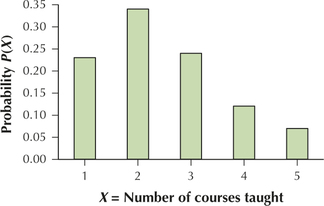
61. Number of Courses Taught. The table provides the probability distribution for X = number of courses taught by faculty at all degree-granting institutions of higher learning in the United States during the fall 2010 semester.1
| ) | |
|---|---|
| 1 | 0.23 |
| 2 | 0.34 |
| 3 | 0.24 |
| 4 | 0.12 |
| 5 | 0.07 |
- Explain why the number of courses taught is a random variable.
- Explain why the number of courses taught is a discrete, and not a continuous, random variable.
- Construct a probability distribution graph for .
- Find .
- Compute .
- Identify the most likely value of .
6.1.61
(a) A faculty member from all degree-granting institutions in the United States is randomly selected. (b) The number of classes taught by a faculty member is counted.
(c)
(d) 0.43 (e) 0.19 (f) 2 classes
Question 6.62
floridacar
62. Florida Vehicle Ownership. The following table provides the probability distribution for X = the number of vehicles owned by residents of Florida. (Note that this data ignores the small number of owners of four or more vehicles.)
| 0 | 0.08 |
| 1 | 0.42 |
| 2 | 0.38 |
| 3 | 0.12 |
- Explain why the number of vehicles owned is a random variable.
- Explain why the number of vehicles owned is a discrete, not a continuous, variable.
- Construct a probability distribution graph for .
- Find .
- Identify the most likely and the least likely numbers of vehicles owned.
Question 6.63
manhattanvehicles
63. Manhattan Car Accidents: Number of Vehicles Involved. The New York City Police Department tracks the number of vehicles involved in each vehicle collision in Manhattan. The table shows the frequency distribution for X = the number of vehicles involved in collisions in Manhattan in July 2014.
| Frequency | |
|---|---|
| 1 | 288 |
| 2 | 3151 |
| 3 | 109 |
| 4 | 12 |
| 5 | 4 |
| 8 | 1 |
- Construct a probability distribution table for .
- Find the probability that at least three vehicles are involved in a collision.
- Find the probability that six vehicles are involved in a collision.
- Find .
- Calculate .
6.1.63
(a)
| 1 | 0.0808 |
| 2 | 0.8839 |
| 3 | 0.0306 |
| 4 | 0.0034 |
| 5 | 0.0011 |
| 8 | 0.0003 |
| Total | 1.0001 |
(b) 0.0354 (c) 0 (d) 0.9953 (e) 0.8839
Question 6.64
64. Manhattan Car Accidents: Number of Injured. The New York City Police Department tracks the number of people injured in each collision that occurs in Manhattan. The table shows the frequency distribution for X = the number of people injured in collisions in Manhattan in July 2014.
| Frequency | |
|---|---|
| 0 | 3028 |
| 1 | 462 |
| 2 | 57 |
| 3 | 10 |
| 4 | 3 |
| 5 | 2 |
| 6 | 1 |
| 7 | 2 |
- Construct a probability distribution table for .
- Find the probability that no one was injured in a collision.
- Use your answer from (b) and the concept of complement (Section 5.2) to find the probability that at least one person was injured in a collision.
- Find .
- Calculate .
Question 6.65
65. Number of Courses Taught. Refer to Exercise 61.
- Find and interpret the expected number of courses.
- Calculate the variance and standard deviation of the number of courses taught.
- Use the -score method to determine whether it is unusual to teach five courses.
6.1.65
(a) The expected number of classes taught is 2.46. (b) classes squared; classes. (c) It is unusual to teach 5 classes.
Question 6.66
66. Florida Vehicle Ownership. Refer to Exercise 62.
- Find and interpret the expected number of vehicles owned.
- Compute the variance and standard deviation of the number of vehicles owned.
- Use the -score method to determine whether it is unusual to own zero vehicles.
Question 6.67
67. Manhattan Car Accidents: Number of Vehicles Involved. Refer to Exercise 63.
- Calculate and interpret the expected value of the number of vehicles involved in a collision.
- Compute the variance and standard deviation of the number of vehicles involved in a collision.
- Use the -score method to identify all unusual or somewhat unusual numbers of vehicles involved in a collision.
6.1.67
(a) The expected number of vehicles involved in a crash is 1.9619 vehicles. (b) vehicle squared; vehicle. (c) 4, 5, and 8 vehicles are outliers. 1 vehicle and 3 vehicles are moderately unusual.
Question 6.68
68. Manhattan Car Accidents: Number of Injured. Refer to Exercise 64.
- Calculate and interpret the expected value of the number of people injured.
- Compute the variance and standard deviation of the number of people injured.
- Use the -score method to identify all unusual or somewhat unusual numbers of people injured in a collision.
The Two-Dice Experiment. Use the following information for Exercises 69–76. Your experiment is to toss a pair of fair dice and find .
Question 6.69
69. Recall the sample space for the two-dice experiment from Figure 3 in Section 5.1 (page 247). Construct the probability distribution table of .
6.1.69
| 2 | 3 | 4 | 5 | 6 | 7 | 8 | 9 | 10 | 11 | 12 | |
| 1/36 | 1/18 | 1/12 | 1/9 | 5/36 | 1/6 | 5/36 | 1/9 | 1/12 | 1/18 | 1/36 |
Question 6.70
70. Graph the probability distribution of , estimating the mean using the balance point method.
Question 6.71
71. Calculate the mean , and compare the result with your estimate from part (b). Interpret the value of .
6.1.71
. The estimate is equal to the actual value. If we were to consider tossing two dice an infinite number of times, the mean sum of the dice would be 7.
Question 6.72
72. Compute the standard deviation of .
Question 6.73
73. Determine whether rolling snake eyes is an unusual result. By symmetry, apply your finding to another value of .
6.1.73
Z-score is −2.07; moderately unusual. By symmetry, so is .
Question 6.74
74. Note that the mean of also happens to be the most likely value of . Does it always happen that the mean of a discrete random variable is the same as the most likely value of that variable? If not, give a counterexample.
Question 6.75
75. Challenger Exercise. Specify the conditions when it is true that the mean of equals the most likely value of .
6.1.75
Symmetric, one mode
Question 6.76
 76. Linear Transformation.What if we add the same unknown amount to each value of ? Describe what would happen to the following, and why:
- The mean of
- The standard deviation of
Question 6.77
nflwins
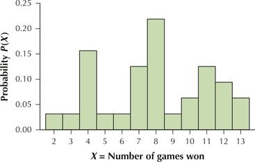
77. National Football League. The number of wins for all 32 teams in the National Football League in the 2013 regular season are given in the table. (Hint: There are many values of in this table. You may wish to use a spreadsheet or other technology to help you solve some of these problems.)
| Team | Wins | Team | Wins |
|---|---|---|---|
| Seattle Seahawks | 13 | Miami Dolphins | 8 |
| Denver Broncos | 13 | Dallas Cowboys | 8 |
| Carolina Panthers | 12 | Chicago Bears | 8 |
| San Francisco 49ers | 12 | Tennessee Titans | 7 |
| New England Patriots | 12 | St. Louis Rams | 7 |
| Indianapolis Colts | 11 | New York Giants | 7 |
| New Orleans Saints | 11 | Detroit Lions | 7 |
| Kansas City Chiefs | 11 | Buffalo Bills | 6 |
| Cincinnati Bengals | 11 | Minnesota Vikings | 5 |
| Arizona Cardinals | 10 | Jacksonville Jaguars | 4 |
| Philadelphia Eagles | 10 | Tampa Bay Buccaneers | 4 |
| San Diego Chargers | 9 | Oakland Raiders | 4 |
| Green Bay Packers | 8 | Atlanta Falcons | 4 |
| Baltimore Ravens | 8 | Cleveland Browns | 4 |
| New York Jets | 8 | Washington Redskins | 3 |
| Pittsburgh Steelers | 8 | Houston Texans | 2 |
- Explain why the number of games is a random variable.
- Explain why the number of games is a discrete, not a continuous random variable.
- Construct a probability distribution table for .
- Draw a probability distribution graph for .
- Find .
- Identify the most likely value of .
6.1.77
(a) An NFL team is selected at random. (b) The number of games a team has won is counted.
(c)
| 2 | 0.0313 |
| 3 | 0.0313 |
| 4 | 0.1563 |
| 5 | 0.0313 |
| 6 | 0.0313 |
| 7 | 0.1250 |
| 8 | 0.2188 |
| 9 | 0.0313 |
| 10 | 0.0625 |
| 11 | 0.1250 |
| 12 | 0.0938 |
| 13 | 0.0625 |
| Total | 1.0004 |
(d)
(e) 0.2502 (f) 8 games won
BRINGING IT ALL TOGETHER
 Chapter 6 Case Study: SAT Scores and AP Exam Scores.
The table contains the frequency distribution of X = score on the Statistics Advanced Placement Exam for students from California. Use this information for Exercises 78–88.
| Frequency | |
|---|---|
| 5 | 3,464 |
| 4 | 5,108 |
| 3 | 6,333 |
| 2 | 4,937 |
| 1 | 6,058 |
| Total |
Question 6.78
APstats
78. Explain why the Statistics AP exam score is a random variable.
Question 6.79
APstats
79. Explain why the Statistics AP exam score is a discrete, not a continuous, variable.
6.1.79
There are finitely many possible exam scores.
Question 6.80
APstats
80. Construct the probability distribution table for X = Statistics AP exam score.
Question 6.81
APstats
81. Confirm that your probability distribution in Exercise 80 is valid.
6.1.81
All probabilities are between 0 and 1 and the probabilities add up to 1.
Question 6.82
APstats
82. Draw a probability distribution graph of .
Question 6.83
APstats
83. Calculate the following probabilities:
- Compare your answers for (a) and (b). Compare your answers for (c) and (d). Explain why this is happening.
6.1.83
(a) 0.7661 (b) 0.7661 (c) 0.4245 (d) 0.4245 (e) Same; Same; is a discrete random variable.
Question 6.84
APstats
84. Calculate the mean Statistics AP exam score, .
Question 6.85
APstats
85. Find the most likely value of .
6.1.85
3
Question 6.86
APstats
86. What is the expected Statistics AP exam score?
Question 6.87
APstats
87. Calculate the variance and standard deviation of .
6.1.87
; .
Question 6.88
APstats
88. Use the -score method to identify any unusual values.
WORKING WITH LARGE DATA SETS
Motor Vehicle Fuel Efficiency. Open the data set FuelEfficiency. We will explore some characteristics of this data set, using the tools and techniques we have learned in this section. Use technology to do Exercises 89–98.
Question 6.89
fuelefficiency
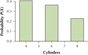
89. Obtain a relative frequency distribution of the variable .
6.1.89
| Relative frequency | |
| 4 | 0.4075 |
| 6 | 0.3637 |
| 8 | 0.2287 |
| Total | 0.9999 |
Question 6.90
fuelefficiency
90. Use the relative frequency distribution in Exercise 89 to construct a probability distribution table of .
Question 6.91
fuelefficiency
91. Construct a probability distribution graph of the number of cylinders.
6.1.91
Question 6.92
fuelefficiency
92. Calculate the mean number of cylinders. Insert this value as the balance point in your probability distribution graph.
Question 6.93
fuelefficiency
93. What is the most likely value of ?
6.1.93
4 cylinders
Question 6.94
fuelefficiency
94. Construct a probability distribution table of .
Question 6.95
fuelefficiency
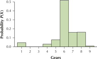
95. Draw a probability distribution graph of .
6.1.95
Question 6.96
fuelefficiency
96. Find the mean number of gears. Insert this value as the balance point in your probability distribution graph.
Question 6.97
fuelefficiency
97. Use a spreadsheet to help you calculate the variance and standard deviation of .
6.1.97
; gears squared; gears.
Question 6.98
fuelefficiency
98. Identify any unusual or somewhat unusual number of gears.