7.2 Section 7.1 Exercises
CLARIFYING THE CONCEPTS
Question 7.1
1. Explain what a sampling distribution is. Why are sampling distributions so important? (p. 396)
7.1.1
It consists of the sample statistics of all possible samples of size n from the population. Sampling distributions can tell us about the expected location and variability of a statistic.
Question 7.2
2. For a normal population, what can we say about the sampling distribution of the sample mean? (p. 399)
Question 7.3
3. True or false: μˉx=μ and σˉx=σ/√n regardless of whether or not the sampling distribution of ˉx is normal. (pp. 397, 398)
7.1.3
True
Question 7.4
4. Use the Central Limit Theorem to explain what happens to the sampling distribution of ˉx as the sample size gets larger. (p. 401)
Question 7.5
5. According to our rule of thumb, what is the minimum sample size for approximate normality of the sampling distribution of ˉx? (p. 401)
7.1.5
n=30
Question 7.6
6. State the three possible cases for the sampling distribution of ˉx. (p. 401)
Question 7.7
7. Suppose we want to decrease the size of the standard error to half its original size. How much do we have to increase the sample size? (p. 398)
7.1.7
4 times as large
Question 7.8
8. State the conditions when the sampling distribution of ˉx is neither normal nor approximately normal. (p. 401)
PRACTICING THE TECHNIQUES
 CHECK IT OUT!
| To do | Check out | Topic |
|---|---|---|
| Exercises 9–16 |
Examples 1 and 2 |
Mean, standard deviation, and shape of the sampling distribution of ˉx |
| Exercises 17–26 | Example 4 | Is the sampling distribution of ˉx normal? |
| Exercises 27–32 | Example 5 | Finding probabilities for the sample mean |
| Exercises 33–58 | Example 6 | Finding a value of ˉx, given a probability or area |
| Exercises 59–70 | Example 7 | Finding probabilities using the Central Limit Theorem for Means |
| Exercises 71–80 | Example 8 | Finding two symmetric sample mean values using the Central Limit Theorem for Means |
| Exercises 81–90 |
Examples 4, 6, and 8 |
When appropriate, calculating two symmetric sample mean values |
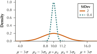
For Exercises 9–16, the characteristics of a normal distribution (X) are given, along with a sample size n for random samples taken from this distribution. Do the following:
- State the value of the mean of the sampling distribution of ˉx, that is, μˉx=μ.
- Calculate the value of the standard error of the sampling distribution of ˉx, that is, σˉx=σ/√n.
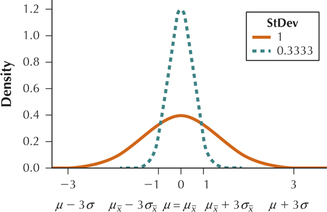
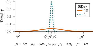
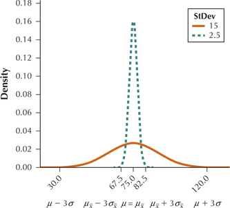
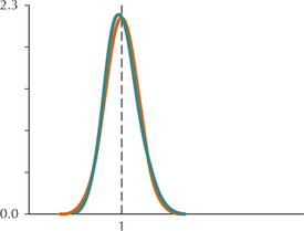
- Draw a graph of the distribution curve of X, similar to the orange curve in Figure 2 on page 398. On the number line, indicate μ, μ-3σ and μ+3σ.
- Draw a graph of the distribution curve for the sampling distribution of ˉx, similar to the green curve in Figure 2 on page 398. On the number line, indicate μˉx, μˉx-3σˉx, and μˉx+3σˉx. Note how both graphs are centered at the population mean, but also note that the variability of the sampling distribution of ˉx is less than that of the original distribution of X.
Question 7.9
9. μ=10,σ=2,n=25
7.1.9
(a) 10 (b) 0.4
(c) and (d)
Question 7.10
10. μ=10,σ=2,n=100
Question 7.11
11. μ=0,σ=1,n=9
7.1.11
(a) 0 (b) 0.3333
(c) and (d)
Question 7.12
12. μ=0,σ=1,n=25
Question 7.13
13. μ=100,σ=10,n=100
7.1.13
(a) 100 (b) 1
(c) and (d)
Question 7.14
14. μ=100,σ=10,n=400
Question 7.15
15. μ=75,σ=15,n=36
7.1.15
(a) 75 (b) 2.5
(c) and (d)
Question 7.16
16. μ=75,σ=15,n=25
For Exercises 17–26, determine whether the sampling distribution of ˉx is normal, approximately normal, or unknown. (Hint: Use the Three Cases on page 401.)
Question 7.17
17. Systolic blood pressure readings are not normally distributed, with μ=78 and σ=7. A random sample of size n=49 is taken.
7.1.17
Approximately normal
Question 7.18
18. Systolic blood pressure readings are not normally distributed, with μ=78 and σ=7. A random sample of size n=25 is taken.
Question 7.19
19. The gas mileage for a 2014 Toyota Prius hybrid vehicle is not normally distributed, with μ=55 miles per gallon and σ=8. A random sample of size n=16 is taken.
7.1.19
Unknown
Question 7.20
20. The gas mileage for a 2014 Toyota Prius hybrid vehicle is not normally distributed, with μ=55 miles per gallon and σ=8. A random sample of size n=64 is taken.
Question 7.21
21. The pollen count distribution for Los Angeles in September is not normally distributed, with μ=10 and σ=2. A random sample of size 16 is taken.
7.1.21
Unknown
Question 7.22
22. The pollen count distribution for Los Angeles in September is not normally distributed, with μ=10 and σ=2. A random sample of size 64 is taken.
Question 7.23
23. Prices for boned trout are normally distributed, with μ=$4.00 per pound and σ=$0.50. A random sample of size 16 is taken.
7.1.23
Normal
Question 7.24
24. Prices for boned trout are not normally distributed, with μ=$4.00 per pound and σ=$0.50. A random sample of size 36 is taken.
Question 7.25
25. Accountant incomes are not normally distributed, with μ=$80,000 per year and σ=$20,000. A random sample of 10 is taken.
7.1.25
Unknown
Question 7.26
26. Accountant incomes are not normally distributed, with μ=$80,000 per year and σ=$20,000. A random sample of 100 is taken.
For Exercises 27–32, assume that test scores (X) follow a normal distribution, with mean μ=100 and standard deviation σ=15. Suppose we take random samples of size n=25.
Question 7.27
27. Calculate μˉx and σˉx.
7.1.27
μˉx=100, σˉx=3
Question 7.28
28. Draw a graph of the sampling distribution of ˉx. On the number line, indicate μˉx,μˉx-3σˉx, and μˉx+3σˉx.
Question 7.29
29. In your graph, shade the area to the left of 97. Find the probability that ˉx is less than 97.
7.1.29
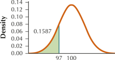
0.1587
Question 7.30
30. In your graph of the sampling distribution of ˉx, shade the area to the left of 98. Is this area smaller or larger than the area in the previous exercise? Will the probability that ˉx is less than 98 be greater than or less than the probability that ˉx is less than 97? Calculate the probability that ˉx is less than 98. Does this confirm your prediction?
Question 7.31
31. Without using your calculator, and referring to the previous exercise, use the symmetry of the normal distribution to calculate the probability that ˉx is greater than 102.
7.1.31
0.2525
Question 7.32
32. Without using your calculator, use your answers from Exercises 30 and 31 to compute the probability that ˉx lies between 98 and 102.
For Exercises 33–38, assume that the random variable X is normally distributed, with mean μ=0 and standard deviation σ=1. We take random samples of size n=100.
Question 7.33
33. Calculate μˉx and σˉx.
7.1.33
μˉx=0, σˉx=0.1
Question 7.34
34. Draw a graph of the sampling distribution of ˉx. On the number line, indicate μˉx,μˉx-3σˉx, and μˉx+3σˉx.
Question 7.35
35. In your graph, shade the area to the right of 0.2. Find the probability that ˉx is greater than 0.2.
7.1.35
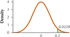
0.0228
Question 7.36
36. Calculate the probability that ˉx exceeds 0.1.
Question 7.37
37. Without using your calculator, and referring to the previous exercise, use the symmetry of the normal distribution to calculate the probability that ˉx is less than –0.1.
7.1.37
0.1587
Question 7.38
38. Without using your calculator, use your answers from Exercises 36 and 37 to compute the probability that ˉx lies between –0.1 and 0.1.
For Exercises 39–46, let the random variable X be normally distributed, with mean μ=10 and standard deviation σ=3. Suppose we take random samples of size n=9. For Exercises 41–46, find the indicated values of ˉx:
Question 7.39
39. Calculate μˉx and σˉx.
7.1.39
μˉx=10, σˉx=1
Question 7.40
40. Draw a graph of the sampling distribution of ˉx. On the number line, indicate μˉx, μˉx-3σˉx, and μˉx+3σˉx.
Question 7.41
41. The value of ˉx greater than 95% of values of ˉx
7.1.41
11.65
Question 7.42
42. The value of ˉx smaller than 95% of values of ˉx
Question 7.43
43. The 97.5th percentile of the sample means
7.1.43
11.96
Question 7.44
44. The 2.5th percentile of the sample means
Question 7.45
45. The two symmetric values for the sample mean that contain the middle 90% of sample means. (Hint: Use your answers to Exercises 41 and 42.)
7.1.45
8.35 and 11.65
Question 7.46
46. The two symmetric values for ˉx that contain the middle 95% of ˉx values. (Hint: Use your answers to Exercises 43 and 44.)
For Exercises 47–52, assume that the random variable X follows a normal distribution, with mean μ=100 and standard deviation σ=15. We take random samples of size n=25.
Question 7.47
47. Calculate μˉx and σˉx.
7.1.47
μˉx=100, σˉx=3
Question 7.48
48. Draw a graph of the sampling distribution of ˉx. On the number line, indicate μˉx, μˉx-3σˉx, and μˉx+3σˉx.
Question 7.49
49. Find the value of ˉx that is greater than 95% of all values of ˉx.
7.1.49
104.95
Question 7.50
50. Without using your calculator, use the symmetry of the normal distribution to calculate the value of ˉx that is smaller than 95% of all values of ˉx.
Question 7.51
51. In your graph, shade the middle 90% of the area under the curve. What are the two symmetric values for the sample mean that contain the middle 90% of sample means?
7.1.51
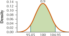
95.05 and 104.95
Question 7.52
52. What proportion of ˉx values lies outside the values you found in the previous exercise?
For Exercises 53–58, assume that the random variable X is normally distributed, with mean μ=0 and standard deviation σ=1. Suppose we take random samples of size n=16.
Question 7.53
53. Calculate μˉx and σˉx.
7.1.53
μˉx=0, σˉx=0.25
Question 7.54
54. Draw a graph of the sampling distribution of ˉx. On the number line, indicate μˉx,μˉx-3σˉx, and μˉx+3σˉx.
Question 7.55
55. Find the value of ˉx that is greater than 97.5% of all values of ˉx.
7.1.55
0.49
Question 7.56
56. Without using your calculator, use the symmetry of the normal distribution to calculate the value of ˉx that is smaller than 97.5% of all values of ˉx.
Question 7.57
57. In your graph, shade the middle 95% of the area under the curve. What are the two symmetric values for the sample mean that contain the middle 95% of sample means?
7.1.57
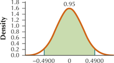
20.49 and 0.49
Question 7.58
58. What proportion of ˉx values lies outside the values you found in the previous exercise?
For Exercises 59–64, assume that X=GPA is not normally distributed with mean μ=2.5 and standard deviation σ=0.5. Suppose we take random samples of size n=100.
Question 7.59
59. Calculate μˉx and σˉx.
7.1.59
μˉx=2.5, σˉx=0.05
Question 7.60
60. Draw a graph of the sampling distribution of ˉx. On the number line, indicate μˉx, μˉx-3σˉx, and μˉx+3σˉx.
Question 7.61
61. In your graph, shade the area to the right of 2.6. Find the probability that ˉx is greater than 2.6.
7.1.61
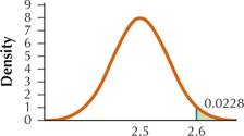
0.0228
Question 7.62
62. Calculate the probability that ˉx exceeds 2.75.
Question 7.63
63. In your graph, shade the area to the left of 2.4. Compute the probability that ˉx is less than 2.4.
7.1.63
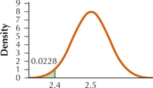
0.0228
Question 7.64
64. Now shade the area between 2.4 and 2.6. Calculate the probability that ˉx lies between 2.4 and 2.6.
For Exercises 65–70, X=golf score is not normally distributed with mean μ=-5 and standard deviation σ=4. Suppose we take random samples of size n=64.
Question 7.65
65. Calculate μˉx and σˉx.
7.1.65
μˉx=−5, σˉx=0.5
Question 7.66
66. Draw a graph of the sampling distribution of ˉx. On the number line, indicate μˉx, μˉx-3σˉx, and μˉx+3σˉx.
Question 7.67
67. In your graph, shade the area to the right of -5.75. Find the probability that ˉx is greater than -5.75.
7.1.67
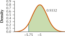
0.9332
Question 7.68
68. In your graph, shade the area to the left of -5.25. Calculate the probability that ˉx is less than -5.25.
Question 7.69
69. Shade the area between -5.75 and -5.75. Would you say that this represents a large probability or a small probability?
7.1.69
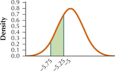
Question 7.70
70. Calculate the probability that the sample mean golf score lies between -5.75 and -5.25.
For Exercises 71–76, X=stats quiz scores has a mean μ=80 and standard deviation σ=6. We take random samples of size n=36.
Question 7.71
71. Calculate μˉx and σˉx.
7.1.71
μˉx=80, σˉx=1
Question 7.72
72. Draw a graph of the sampling distribution of ˉx. On the number line, indicate μˉx, μˉx-3σˉx, and μˉx+3σˉx.
Question 7.73
73. Find the value of ˉx that is greater than 99.5% of all values of ˉx.
7.1.73
82.58
Question 7.74
74. Without using your calculator, use the symmetry of the normal distribution to calculate the value of ˉx that is smaller than 99.5% of all values of ˉx.
Question 7.75
75. In your graph, shade the middle 99% of the area under the curve. What are the two symmetric values for the sample mean that contain the middle 99% of sample means?
7.1.75
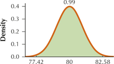
77.42 and 82.58
Question 7.76
76. What proportion of ˉx values lies outside the values you found in the previous exercise?
For Exercises 77–80, X=baseball scores has a mean μ=5 and standard deviation σ=2. Suppose we take random samples of size n=64.
Question 7.77
77. Calculate μˉx and σˉx.
7.1.77
μˉx=5, σˉx=0.25
Question 7.78
78. Draw a graph of the sampling distribution of ˉx. On the number line, indicate μˉx, μˉx-3σˉx, and μˉx+3σˉx.
Question 7.79
79. In your graph, shade the middle 95% of the area under the curve. What are the two symmetric values for the sample mean that contain the middle 95% of sample means?
7.1.79
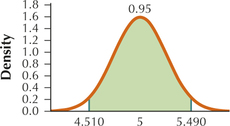
4.51 and 5.49
Question 7.80
80. What proportion of ˉx values lies outside the values you found in the previous exercise?
For the situations in Exercises 81–90, if possible, find the indicated two symmetric values of ˉx that contain the middle 95% of sample means. If not possible, explain why not.
Question 7.81
81. The pollen count distribution for Los Angeles in September is not normally distributed, with μ=10 and σ=2. Random samples of size n=16 are taken.
7.1.81
Not possible; variable not normally distributed and sample size less than 30
Question 7.82
82. The pollen count distribution for Los Angeles in September is not normally distributed, with μ=10 and σ=2. Random samples of size n=64 are taken.
Question 7.83
83. Prices for boned trout are normally distributed, with μ=$4.00 per pound and σ=$0.50. Random samples of size n=16 are taken.
7.1.83
$3.755 and $4.245
Question 7.84
84. Prices for boned trout are not normally distributed, with μ=$4.00 per pound and σ=$0.50. Random samples of size n=9 are taken.
Question 7.85
85. Accountant incomes are not normally distributed, with μ=$80,000 per year and σ=$20,000. Random samples of size n=10 are taken.
7.1.85
Not possible; variable not normally distributed and sample size less than 30
Question 7.86
86. Accountant incomes are normally distributed, with μ=$80,000 per year and σ=$20,000. Random samples of size n=100 are taken.
Question 7.87
87. Systolic blood pressure readings are not normally distributed, with μ=78 and σ=7. Random samples of size n=49 are taken.
7.1.87
76.04 and 79.96
Question 7.88
88. Systolic blood pressure readings are not normally distributed, with μ=78 and σ=7. Random samples of size n=25 are taken.
Question 7.89
89. The gas mileage for a 2014 Toyota Prius hybrid vehicle is not normally distributed, with μ=55 miles per gallon and σ=8. Random samples of size n=16 are taken.
7.1.89
Not possible; variable not normally distributed and sample size less than 30
Question 7.90
90. The gas mileage for a 2014 Toyota Prius hybrid vehicle is not normally distributed, with μ=55 miles per gallon and σ=8. Random samples of size n=64 are taken.
APPLYING THE CONCEPTS
Question 7.91
91. Blood Lead Contamination. A study2 of workers in lead-exposed jobs found that the mean blood lead level was μ=31.4 micrograms, with a standard deviation of σ=14.2 micrograms. Let the sample size be n=16. Assume the distribution is normal.
- Find the mean of the sampling distribution μˉx and the standard error σˉx.
- Calculate the probability that the sample mean blood lead level will be less than 27.85 micrograms.
- Compute P(ˉx>38.5).
7.1.91
(a) μˉx=31.4 micrograms, σˉx=3.55 micrograms (b) 0.1587
(c) 0.0228
Question 7.92
92. Student Debt. The Project on Student Debt published a study3 in which they found that the mean amount of student debt owed by American college students was μ=$29,400. Assume a standard deviation of σ=$9000. Suppose we take a sample of n=9 students. Assume the distribution is normal.
- Find the mean of the sampling distribution μˉx and the standard error σˉx.
- Calculate the probability that the sample mean student debt will be greater than $32,400.
- Compute P(ˉx<$24,900).
Question 7.93
93. Measuring Well-Being. The Gallup-Healthways Well-Being Index represents an average of the reported emotional health, physical health, healthy behavior, and work environment of the survey respondents.4 Gallup reported that the mean Well-Being Index in 2013 was μ=66.2. Assume the standard deviation was σ=10. Suppose we take a sample of 25 survey respondents. If we assume the underlying distribution is normal, find the probability that the sample mean Well-Being Index will have the following values:
- Greater than 76.2
- Between 56.2 and 76.2
- Less than 56.2
7.1.93
(a) Approximately 0 (b) Approximately 1 (c) Approximately 0
Question 7.94
94. Statisticians' Salaries. If you enjoy statistics, you may want to become a statistician. The U.S. Census Bureau reported in 2014 that the median salary for mathematicians and statisticians was about $86,000. Income data is usually right-skewed, so we may safely assume that the mean is higher. Suppose the salaries of statisticians have a mean of μ=$100,000 and a standard deviation of σ=$20,000.
Suppose we take samples of size 100 statisticians. Find the probability that the sample mean salary will have the following values:
- More than $106,000
- Less than $90,000
- Between $90,000 and $106,000
Question 7.95
95. Blood Lead Contamination. Refer to Exercise 91.
- Find the sample mean blood lead level greater than 95% of all sample mean blood lead levels.
- Find the value of ˉx smaller than 95% of all sample mean blood lead levels.
- What are the two symmetric values of ˉx that contain the middle 90% of sample means?
7.1.95
(a) 37.2575 micrograms (b) 25.5425 micrograms (c) 25.5425 micrograms and 37.2575 micrograms
Question 7.96
96. Student Debt. Refer to Exercise 92.
- Find the sample mean student debt greater than 97.5% of all sample mean student debts.
- Find the value of ˉx smaller than 97.5% of all sample mean student debts.
- What are the two symmetric values of ˉx that contain the middle 95% of sample means?
Question 7.97
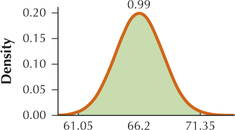
97. Measuring Well-Being. Refer to Exercise 93.
- What are the two symmetric values of ˉx that contain the middle 99% of sample means?
- Draw a graph of the sampling distribution of ˉx, showing μˉx, along with the two symmetric values of ˉx from part (a). Shade the area under the curve between these two values of ˉx, and indicate the amount of area this represents.
7.1.97
(a) 61.05 and 71.35
(b)
Question 7.98
98. Statisticians' Salaries. Refer to Exercise 94.
- What are the two symmetric values of ˉx that contain the middle 80% of sample means?
- Draw a graph of the sampling distribution of ˉx, showing μˉx, along with the two symmetric values of ˉx from part (a). Shade the area under the curve between these two values of ˉx, and indicate the amount of area this represents.
Question 7.99
99. Cholesterol Levels. The Centers for Disease Control and Prevention reports that the mean serum cholesterol level in Americans is 202. Assume that the standard deviation is 45. There is no information about the distribution. We take a sample of 36 Americans.
- Find P(ˉx>212).
- Calculate P(192<ˉx<212).
7.1.99
(a) 0.0918 (TI-83/84: 0.0912) (b) 0.8164 (TI-83/84: 0.8176)
Question 7.100
100. Tennessee Temperatures. According to the National Oceanic and Atmospheric Administration, the mean temperature for Nashville, Tennessee, in the month of January between 1872 and 2014 was 38.6°F. Assume that the standard deviation is 10°F, but the distribution is unknown. If we take a sample of n=36, find the following probabilities:
- P(ˉx<40)
- P(40<ˉx<41)
Question 7.101
101. Computers per School. The National Center for Educational Statistics (http://nces.ed.gov) reported that the mean number of instructional computers per public school nationwide was 124. Assume that the standard deviation is 50 computers and no information is available about the shape of the distribution. Suppose we take a sample of size 100 public schools. Compute the following probabilities:
- P(ˉx<110)
- P(110<ˉx<124)
7.1.101
(a) 0.0026 (b) 0.4974
Question 7.102
102. Cholesterol Levels. Refer to Exercise 99.
- Find the sample mean serum cholesterol level that is larger than 95% of all such sample means.
- Calculate the sample mean serum cholesterol level that is smaller than 95% of all such sample means.
Question 7.103
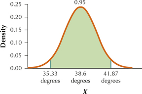
103. Tennessee Temperatures. Refer to Exercise 100.
- Find the sample mean temperature that is larger than 97.5% of all such sample means.
- Calculate the sample mean temperature that is smaller than 97.5% of all such sample means.
- Draw a graph of the sampling distribution of ˉx. Indicate μˉx, the two ˉx values from (a) and (b), and the area between them.
7.1.103
(a) 41.87 (b) 35.33
(c)
Question 7.104
104. Computers per School. Refer to Exercise 101.
- Find the 0.5th percentile of sample mean numbers of computers.
- Compute the 99.5th percentile of sample mean numbers of computers.
- Draw a graph of the sampling distribution of ˉx. Indicate μˉx, the two ˉx values from (a) and (b), and the area between them.
Question 7.105
105. Carbon Dioxide Concentration. The Carbon Dioxide Information Analysis Center (cdiac.ornl.gov/pns/current_ghg.html) reported in 2014 that the mean concentration of the greenhouse gas carbon dioxide is 397 parts per million (ppm). Suppose the population is normally distributed, assume that the standard deviation is 25 ppm, and suppose we take atmospheric samples from 25 cities.
- Calculate the probability that the sample mean carbon dioxide concentration will be between 387 and 407 ppm.
- Which sample mean represents the median sample mean? Explain how you know this.
- Find the two symmetric sample mean carbon dioxide concentrations containing the middle 99% of all sample means.
7.1.105
(a) 0.9544 (b) 397 ppm; in a normal distribution the median equals the mean. (c) 384.12 ppm and 409.88 ppm
Question 7.106
106. Short-Term Memory. In a famous research paper in the psychology literature, George Miller found that the amount of information humans could process in short-term memory was 7 bits (pieces of information), plus or minus 2 bits.5 Assume that the mean number of bits is 7 and the standard deviation is 2, and that the distribution is normal. Suppose we take a sample of 100 people and test their short-term memory skills.
- Find the probability that the sample mean number of bits retained in short-term memory lies between 6.8 and 7.2.
- Between which two values do the middle 95% of sample mean number of bits retained in short-term memory lie?
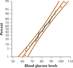
Blood Glucose Levels. Use the following information for Exercises 107–109. The population mean blood glucose levels is μ=80 with standard deviation σ=10. Here is the normal probability plot for the population of patients.
Question 7.107
107. Does the normal probability plot show evidence in favor of normality or against normality? What characteristics of the plot illustrate this evidence?
7.1.107
In favor of normality. All of the points are between the curved lines and most of the points are close to the center line.
Question 7.108
108. If possible, find the probability that a random sample of n=9 patients will have a mean blood glucose level greater than 86. If not possible, explain why not.
Question 7.109
109. If possible, find the probability that a random sample of n=36 patients will have a mean blood glucose level greater than 86. If not possible, explain why not.
7.1.109
0 (TI-83/84: 0.0001591)
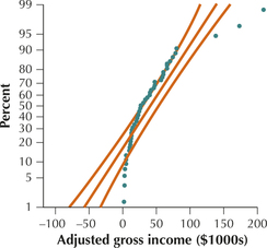
Adjusted Gross Income. Use the following information for Exercises 110–113. The population mean adjusted gross income for instructors at a certain college is μ=$50,000 with standard deviation σ=$30,000. Here is the normal probability plot for the population of instructors.
Question 7.110
110. Does the normal probability plot show evidence in favor of normality or against normality? What characteristics of the plot illustrate this evidence?
Question 7.111
111. If possible, find the probability that a random sample of n=16 instructors will have a mean adjusted gross income between $40,000 and $60,000. If not possible, explain why not.
7.1.111
Not possible. The variable is not normally distributed and the sample size is less than 30.
Question 7.112
112. If possible, find the probability that a random sample of n=36 instructors will have a mean adjusted gross income between $40,000 and $60,000. If not possible, explain why not.
Question 7.113
 113. Refer to Exercise 112. What if the sample size used was some unspecified value greater than 36? Describe how and why this change would have affected the following, if at all. Would the quantities increase, decrease, remain unchanged? Or is there insufficient information to tell what would happen? Explain your answers.
- μˉx
- σˉx
- Z=ˉx-μˉxσˉx
- P($40,000 <ˉx<$60,000)
7.1.113
(a) Remain unchanged. From Fact 1 in Section 7.1, μˉx=μ. Thus μˉx does not depend on the sample size n. (b) Decrease. Since σˉx=σ/(√n),, an increase in the sample size n results in a decrease in σˉx. (c) Insufficient information to tell. If ˉx>50,000, then ˉx−50,000>0. Since σˉx decreases and is positive, Z=(x−μˉx)/σˉx will increase. If ˉx=50,000, then ˉx−50,000=0. Thus Z=(x−μˉx)/σˉx will remain 0. If ˉx<50,000, then ˉx−50,000<0. Since σˉx decreases and is positive, Z=(x−μˉx)/σˉx will decrease. (d) Increase. From part (c), Z=(x−μˉx)/σˉx=(60,000−50,000)/σx will increase and Z=(x−μˉx)/σˉx=(40,000−50,000)/σx will decrease. Thus the area between these two values will increase. Since P($40,000<ˉx<$60,000) is the area between these two values of Z,P($40,000<ˉx<$60,000) will increase.
 Chapter 7 Case Study: Trial of the Pyx. Refer to the Case Study on pages 407, 408, and 409 for Exercises 114, 115, 116, 117, and 118.
Question 7.114
114. What were the chances that the Master of the Mint would have been accused of cheating if he had in fact been completely honest?
In the Case Study, we interpreted the phrase “much less than” to mean a measurement that is 2 or more standard deviations below the mean. For Exercises 115–118, suppose we interpret the phrase “much less than” to mean a measurement that is 3 or more standard deviations below the mean.
Question 7.115
115. Use the methods shown in the Case Study to answer the following questions:
- What would be the new value of σˉx?
- What would be the standard deviation s for each gold piece?
- By the Empirical Rule, about what proportion of the mean weights would you now expect to lie between 127.68 and 128.32?
7.1.115
(a) 0.1067 gram (b) 1.067 grams (c) About 0.997
Question 7.116
116. Assume “just a little debasement” from 128 grams per coin to 127.9 grams per coin.
- Find P(127.68<ˉx<128.32).
- What is the probability that the Master of the Mint would get away with just this little debasement? That he would get caught?
- Compare the probabilities in (b) with those in the Case Study in the text. Which values favor the Master of the Mint?
Question 7.117
117. Assume that greed attacked the Master of the Mint and he went for the big debasement from 128 grams per coin to 127.3 grams per coin.
- Find P(127.68<ˉx<128.32).
- What is the probability that the Master of the Mint would get away with this big debasement? That he would get caught?
- Compare the probabilities in (b) with those in the Case Study in the text. Which values favor the Master of the Mint?
7.1.117
(a) 0.0002 (b) 0.0002, 0.9998 (c) The value found in the original case study in the text favors the Master of the Mint.
Question 7.118
118. The Master of the Mint wanted to choose a mean value so that his chances of failing the Trial of the Pyx were 25%. Which mean value is this?
![]() Use the Central Limit Theorem applet for Exercises 119 and 120.
Use the Central Limit Theorem applet for Exercises 119 and 120.
Question 7.119
119. Describe the shape of the sampling distribution of ˉx for the following sample sizes:
- 2
- 5
- 30
7.1.119
(a) n=2
(b) n=5
(c) n=30
Question 7.120
120. At what sample size would you say the sampling distribution of ˉx becomes approximately normal?
BRINGING IT ALL TOGETHER
SAT Math Scores. Use this information for Exercises 121–126. The College Board (www.collegeboard.com) reports that the nationwide mean math SAT score for 2013 is 514. Assume that the standard deviation is 116 and that the scores are normally distributed.
Question 7.121
121. What is the probability that a randomly selected SAT Math score will be less than 500?
7.1.121
0.4522
Question 7.122
122. As a researcher, you are looking at samples of SAT Math scores of size 16.
- Find μˉx.
- Find σˉx.
- What can you say about the sampling distribution of the sample mean? How do you know this?
Question 7.123
123. Refer to Exercise 122.
- What is the probability that a sample of 16 students will have a sample mean math SAT score below 500?
- Why is the probability so much lower for the sample mean than for a particular student?
7.1.123
(a) 0.3156 (b) Means are less variable than individual values.
Question 7.124
124. Calculate the following sample mean values:
- 99.5th percentile of the sample mean SAT Math scores
- 0.5th percentile of the sample mean SAT Math scores
Question 7.125
125. Refer to Exercise 123. What if the population standard deviation was greater than 116? Explain how this would affect the following, if at all:
- Probability that a randomly selected SAT Math score will be less than 500
- μˉx
- σˉx
- Sampling distribution of the sample mean
7.1.125
(a) Increase (b) Remain the same (c) Increase (d) Still normal with μˉx=514 but σˉx would increase
Question 7.126
126. What if the population standard deviation was greater than 116? Explain how this would affect the following, if at all:
- Probability that a sample of 16 SAT Math scores will have a mean less than 500
- 99.5th percentile of the sample mean SAT Math scores
- 0.5th percentile of the sample mean SAT Math scores