9 Hypothesis Testing

9.2 $Z$ Test for the Population Mean: Critical-Value Method

OBJECTIVES By the end of this section, I will be able to …

Explain the essential idea about hypothesis testing for the population mean.
Calculate the test statistic $Z_{data}$ .
Find the critical region(s) and critical value(s) for a hypothesis test.
Perform the $Z$ test for the mean, using the critical-value method.

1 The Essential Idea About Hypothesis Testing for the Mean

Recall that in Section 9.1, we wanted to determine whether the population mean systolic blood pressure $μ$ was less than 110 and we considered the hypotheses

$H_{0} : μ = 110 versus H_{a} : μ < 110$

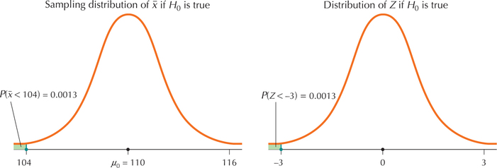
We stated that a large difference between the observed sample mean $\bar{x}$ and the hypothesized mean $μ_{0} = 110$ would result in the rejection of the null hypothesis $H_{0}$ . The question is, “How large is large?”

The $Z$ test for the mean tells us when our results are statistically significant. To learn how this test works, consider the following: A sample of $n = 25$ patients who are taking the medication shows a sample mean systolic blood pressure level of $\bar{x} = 104$ . Further assume that the population standard deviation systolic blood pressure reading is $σ = 10$ , and that the population of such readings is normal. Would this value $\bar{x} = 104$ represent sufficient evidence to reject $H_{0}$ and conclude that $μ < 110$ ?

Recall from Chapter 7 that the sampling distribution of the sample mean $\bar{x}$ is the collection of sample means of all possible samples of size $n$ . When the population is normal, or the sample size is large, the sampling distribution of $\bar{x}$ is approximately normal, with mean $μ_{\bar{x}} = μ$ and standard error $σ_{\bar{x}} = σ / \sqrt{n}$ . The idea behind the $Z$ test is to determine where our sample mean $\bar{x} = 104$ falls within the sampling distribution. Is $\bar{x} = 104$ somewhere near the middle of the sampling distribution, or is it an outlier? Now, if $H_{0}$ is true, then $μ = μ_{0} = 110$ and we may standardize $\bar{x}$ to get

Page 498

$Z = \frac{\bar{x} - μ_{0}}{σ / \sqrt{n}}$

Substituting, we get

$Z = \frac{\bar{x} - μ_{0}}{σ / \sqrt{n}} = \frac{104 - 110}{10 / \sqrt{25}} = - 3$

In other words, $\bar{x} = 104$ lies 3 standard errors below the hypothesized mean $μ_{0} = 110$ . Thus, if we accept that the null hypothesis is true, then $\bar{x} = 104$ is an outlier, an extreme value (see Figure 1). That is, if $H_{0}$ is true, then the probability of observing $\bar{x} \leq 104$ is very small $(P (Z < - 3) = 0.0013)$ , because the corresponding $Z$ -value lies in the tail of the distribution, and nearly all the values of $\bar{x}$ are greater than 104.

Note: Here, we are using Facts 1–4 and the Central Limit Theorem from Chapter 7.

We are developing the $Z$ test using a left-tailed test, but the same idea applies to right-tailed tests and twotailed tests, too.

FIGURE 1 An extreme value of

$\bar{x}$ calls for rejection of

$H_{0}$ .

Thus, we must choose one of the following two scenarios:

$H_{0}$ is true, the value of $μ_{0}$ is accurate, and our observation of this extreme value of $\bar{x}$ is an amazingly unlikely event.
$H_{0}$ is not correct, and the true value of $μ$ is closer to $\bar{x}$ .

Developing Your Statistical Sense

The Data Prevail!

When faced with the above situation, because we don't want to base our decisions on “amazingly unlikely events,” we therefore would conclude that $H_{0}$ is not correct. Remember that the null hypothesis is just a conjecture, but the sample mean $\bar{x}$ represents directly observable “hard data.” The scientific method states that, when there is a conflict between a conjecture and the observed data, the data prevail, and we need to rethink our null hypothesis.

This conclusion illustrates the essential idea about hypothesis testing for the mean.

The Essential Idea About Hypothesis Testing for the Mean

When the observed value of $\bar{x}$ is unusual or extreme in the sampling distribution of $\bar{x}$ that assumes $H_{0}$ is true, we should reject $H_{0}$ . Otherwise, we should not reject $H_{0}$ .

All the remaining parts of Sections 9.2–9.4, all the steps and all the calculations, are really just ways to implement this essential idea. Stated roughly: If the difference between $\bar{x}$ and $μ_{0}$ is large, then reject $H_{0}$ . Otherwise don't.

Page 499

2 Test Statistic $Z_{data}$

The $Z$ statistic that we calculated earlier

$Z = \frac{\bar{x} - μ_{0}}{σ / \sqrt{n}}$

contains four quantities—three of which are taken from data. The sample mean $\bar{x}$ and the sample size $n$ are characteristics of the sample data, and the population standard deviation σ represents the population data. Thus, we call this statistic $Z_{data}$ .

The Test Statistic $Z_{data}$

The test statistic used for the $Z$ test for the mean is

$Z_{data} = \frac{\bar{x} - μ_{0}}{σ / \sqrt{n}}$

$Z_{data}$ summarizes the information in the data set regarding the hypothesis test.

For the blood pressure data, we have

$Z_{data} = \frac{\bar{x} - μ_{0}}{σ / \sqrt{n}} = \frac{104 - 110}{10 / \sqrt{25}} = - 3$

$Z_{data}$ is an example of a test statistic, a statistic generated from a data set for the purposes of testing a statistical hypothesis. We will discuss several other test statistics throughout the remainder of the text. The hypothesis test in this section and Section 9.3 is called the Z test because the test statistic $Z_{data}$ comes from the standard normal $Z$ distribution.

EXAMPLE 7 Calculating $Z_{data}$

Clothing Store Sales

Retail stores need to generate sales. A sample of 100 customers' data was taken from the Chapter 9 Case Study data set, Clothing Store, and the total sales were obtained for each customer during the six-month time period. Suppose this sample showed a sample mean of $\bar{x} = $ 480$ . Assume the population standard deviation is $σ = $ 670$ . The district manager has set a goal to achieve a population mean of more than $413 total sales per customer.

Construct the hypotheses.
Calculate the test statistic $Z_{data}$ .

Solution

Using our strategy for constructing the hypotheses from Section 9.1, the key words “more than” means “>,” and the “>” symbol occurs only in the right-tailed test. Answering the question “More than what?” is $μ_{0} = 413$ . Thus, our hypotheses are

$H_{0} : μ = 413 versus H_{a} : μ > 413$

where $μ$ represents the population mean total sales per customer.
The sample size is $n = 100$ , with a sample mean of $\bar{x} = 480$ , and $σ = 670$ . Thus,

$Z_{data} = \frac{\bar{x} - μ_{0}}{σ / \sqrt{n}} = \frac{480 - 413}{670 / \sqrt{100}} = 1$

NOW YOU CAN DO

Exercises 9–22.

YOUR TURN#3

For Example 7, suppose everything else stayed the same, but now $n = 36$ . Calculate $Z_{data}$ .

(The solution is shown in Appendix A.)

Page 500

$Z_{data}$ standardizes the distance between the sample mean $\bar{x}$ and the hypothesized population mean $μ$ , so that this distance is now on the standard normal scale. Thus, we can sometimes tell with a glance at $Z_{data}$ , using our knowledge of the standard normal $Z$ distribution (Section 6.4), whether $\bar{x}$ is extreme or not, and therefore whether to reject. Specifically, we recall that almost all values of $Z$ lie between −3 and 3. Here are two examples:

Say our data provides us with a value of $Z_{data} = 12$ , which is far into the tail of the $Z$ distribution. This represents a very extreme value of $\bar{x}$ , and so we will reject $H_{0}$ .
Suppose the data set gives us a value of $Z_{data} = 0.27$ , which is near the center of the $Z$ distribution. This represents a value of $\bar{x}$ fairly close to $μ_{0}$ , and so we will not reject $H_{0}$ .

Of course, not all cases are as obvious as these, thus the need for the hypothesis testing procedure.

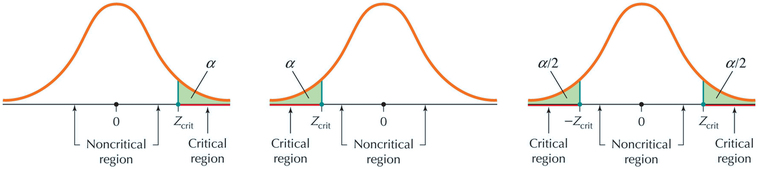
3 Critical Regions and Critical Values

In the critical-value method for the $Z$ test, we compare $Z_{data}$ with a threshold value, or critical value of $Z$ , called $Z_{crit}$ . The value of $Z_{crit}$ separates $Z$ into two regions (see Table 4):

Critical region: the values of $Z_{data}$ for which we reject $H_{0}$
Noncritical region: the values of $Z_{data}$ for which we do not reject $H_{0}$

The critical region consists of the range of values of the test statistic $Z_{data}$ for which we reject the null hypothesis.
The noncritical region consists of the range of values of the test statistic $Z_{data}$ for which we do not reject the null hypothesis.
The value of $Z$ that separates the critical region from the noncritical region is called the critical value $Z_{crit}$ .

$Z_{crit}$ represents the boundary between values of $Z_{data}$ that are statistically significant and those that are not statistically significant. The value of $Z_{crit}$ depends on the value of $α$ , the probability of wrongly rejecting $H_{0}$ . A smaller value of $α$ will make it harder to reject $H_{0}$ , that is, harder to find statistical significance. Thus, $α$ is called the level of significance of the hypothesis test.

The value of $Z_{crit}$ depends on (a) the form of the hypothesis test, and (b) the level of significance $α$ . Table 4 shows values of $Z_{crit}$ for the most commonly used levels of significance $α$ . It also shows the location of the critical region.

Table 9.7: Table 4 Table of critical values

$Z_{crit}$ for common values of the level of significance

$α$

	Form of hypothesis test
	Right-tailed	Left-tailed	Two-tailed
Level of significance $α$	$H_{0} : μ = μ_{0}$	$H_{0} : μ = μ_{0}$	$H_{0} : μ = μ_{0}$
Level of significance $α$	$H_{a} : μ > μ_{0}$	$H_{a} : μ < μ_{0}$	$H_{a} : μ \neq μ_{0}$
0.10	$Z_{crit} = 1.28$	$Z_{crit} = - 1.28$	$Z_{crit} = 1.645$
0.05	$Z_{crit} = 1.645$	$Z_{crit} = - 1.645$	$Z_{crit} = 1.96$
0.01	$Z_{crit} = 2.33$	$Z_{crit} = - 2.33$	$Z_{crit} = 2.58$
Critical region
Rejection rule:	Reject $H_{0}$ if $Z_{data} \geq Z_{crit}$	Reject $H_{0}$ if $Z_{data} \leq Z_{crit}$	Reject $H_{0}$ if $Z_{data} \leq - Z_{crit}$ or $Z_{data} \geq Z_{crit}$

Page 501

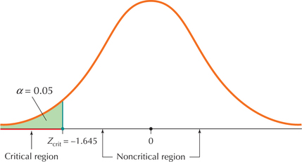
EXAMPLE 8 Finding $Z_{crit}$ and the critical region

For the hypotheses,

$H_{0} : μ = 110 versus H_{a} : μ < 110$

where $μ$ represents the population mean systolic blood pressure, let the level of significance $α = 0.05$ .

Find the critical value $Z_{crit}$ .
Graph the distribution of $Z$ , showing the critical region.

Solution

We have a left-tailed test and level of significance $α = 0.05$ , so Table 4 tells us that the critical value is $Z_{crit} = - 1.645$ . The graph showing the critical region is provided in Figure 2. We would reject $H_{0}$ for values of $Z_{data}$ that are $\leq Z_{crit} = - 1.645$ .

FIGURE 2 Critical region for a left-tailed test lies in the left (lower) tail.

NOW YOU CAN DO

Exercises 23–26.

YOUR TURN#4

In Example 7, we had the hypothesis test:

$H_{0} : μ = 413 versus H_{a} : μ > 413$

where $μ$ represents the population mean total sales per customer. Let the level of significance $α = 0.10$ .

Find the critical value $Z_{crit}$ .
Graph the distribution of $Z$ , showing the critical region.

(The solutions are shown in Appendix A.)

Developing Your Statistical Sense

Why Is It Called a Left-Tailed Test Mean? Right-Tailed Test? Two-Tailed Test?

A hypothesis test of the form

$H_{0} : μ = μ_{0} versus H_{α} : μ < μ_{0}$

is called a left-tailed test because the critical region lies in the left (lower) tail. Similarly, a hypothesis test of the form

$H_{0} : μ = μ_{0} versus H_{α} : μ > μ_{0}$

is called a right-tailed test because its critical region lies in the right (upper) tail. Finally, a hypothesis test of the form

$H_{0} : μ = μ_{0} versus H_{α} : μ \neq μ_{0}$

is called a two-tailed test because its critical region occupies both the lower and upper tails.

Page 502

4 Performing the $Z$ test for the Mean Using the Critical-value Method

We are now ready to learn the steps for performing the $Z$ test for the population mean using the critical-value method.

$Z$ Test for the Population Mean $μ$ : Critical-Value Method

When a random sample of size $n$ is taken from a population where the population standard deviation σ is known, you can use the $Z$ test if (a) the population is normal, or (b) the sample size is large $(n \geq 30)$ .

Step 1 State the hypotheses.

Use one of the forms from Table 4. State the meaning of $μ$ .
Step 2 Find $Z_{crit}$ and state the rejection rule.

Use Table 4 and the given level of significance $α$ .
Step 3 Calculate $Z_{data}$ .

$Z_{data} = \frac{\bar{x} - μ_{0}}{σ / \sqrt{n}}$
Step 4 State the conclusion and the interpretation.

If $Z_{data}$ falls in the critical region, then reject $H_{0}$ ; otherwise, do not reject $H_{0}$ . Interpret your conclusion.

What Does This Conclusion Mean?

Interpreting Your Conclusion

Recall that a data analyst needs to interpret the results so that the general public can understand them. You can use the following generic interpretation for the two possible conclusions. Just remember that generic interpretations are no substitute for thinking clearly about the problem and the implications of the conclusion.

Interpreting the Conclusion

If you reject $H_{0}$ , the interpretation is: There is evidence at level of significance $α$ that [whatever $H_{a}$ says].
If you do not reject $H_{0}$ , the interpretation is: There is insufficient evidence at level of significance $α$ that [whatever $H_{a}$ says].

For example, suppose our conclusion for the hypotheses in Example 8

$H_{0} : μ = 110 versus H_{a} : μ < 110$

was to reject $H_{0}$ . Then the interpretation of this conclusion would be: There is evidence at level of significance $α = 0.05$ that the population mean systolic blood pressure reading is less than 110.

Next, we illustrate the critical-value method of performing a right-tailed $Z$ test, a left-tailed $Z$ test, and a two-tailed $Z$ test for $μ$ .

EXAMPLE 9 $Z$ Test for $μ$ , critical-value method, right-tailed test

Clothing Store Sales

For the situation in Example 7, test at level of significance $α = 0.01$ whether the population mean total sales per customer is more than $413.

Solution

We may apply the $Z$ test because the sample is large $(n \geq 30)$ , and the population standard deviation σ is known.

Page 503

Step 1 State the hypotheses.

From Example 7, our hypotheses are

$H_{0} : μ = 413 versus H_{a} : μ > 413$

where $μ$ represents the population mean total sales per customer.

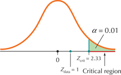FIGURE 3 Critical region for a right-tailed test.
Step 2 Find $Z_{crit}$ and state the rejection rule.

We have a right-tailed test and level of significance $α = 0.01$ , which, from Table 4, tell us that $Z_{crit} = 2.33$ . Because we have a right-tailed test, the rejection rule will be “Reject $H_{0}$ if $Z_{data} \geq Z_{crit}$ ,” that is, “Reject $H_{0}$ if $Z_{data} \geq 2.33$ ” (see Figure 3).
Step 3 Find $Z_{data}$ .

From Example 7, we have $Z_{data} = 1$ .
Step 4 State the conclusion and interpretation.

Our rejection rule states that we will reject $H_{0}$ if $Z_{data} \geq 2.33$ . Because $Z_{data} = 1$ , which is not ≥ 2.33, the conclusion is to not reject $H_{0}$ (Figure 4). Even though the sample mean of $\bar{x} = 480$ exceeds $μ_{0} = 413$ , it does not do so by a wide enough margin to overcome the reasonable doubt that the difference between $\bar{x}$ and $μ_{0}$ may have been due to chance. We interpret our conclusion as follows: “There is insufficient evidence at the 0.01 level of significance that the population mean total sales is greater than $413 per customer over the six-month period.”

NOW YOU CAN DO

Exercises 37–40.

EXAMPLE 10 $Z$ Test for $μ$ , critical-value method, left-tailed test

For the hypotheses in Example 8, perform the $Z$ test for the population mean, using level of significance $α = 0.05$ . Assume systolic blood pressure is normally distributed.

Solution

We may use the $Z$ test, because the population of systolic blood pressure readings is normally distributed, and the population standard deviation σ is known.

Step 1 State the hypotheses.

From Example 8, we have

$H_{0} : μ = 110 versus H_{a} : μ < 110$

where $μ$ represents the population mean systolic blood pressure reading.

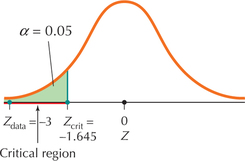FIGURE 4 Critical region for a left-tailed test.
Step 2 Find $Z_{crit}$ and state the rejection rule.

Example 8 gives us the critical value $Z_{crit} = - 1.645$ , and Table 4 tells us that, for level of significance $α = 0.05$ , we will reject $H_{0}$ if $Z_{data} \leq Z_{crit}$ , that is, if $Z_{data} \leq - 1.645$ (Figure 4).
Step 3 Calculate $Z_{data}$ .

From page 499, we know that

$Z_{data} = \frac{\bar{x} - μ_{0}}{σ / \sqrt{n}} = \frac{104 - 110}{10 / \sqrt{25}} = - 3$
Step 4 State the conclusion and the interpretation.

In Step 2, we stated that we would reject $H_{0}$ if $Z_{data} \leq - 1.645$ . Our $Z_{data}$ of $- 3 \leq - 1.645$ , therefore, we reject $H_{0}$ . Our interpretation is: “There is evidence at level of significance $α = 0.05$ that the population mean systolic blood pressure reading is less than 110.”

NOW YOU CAN DO

Exercises 41–44.

Page 504

EXAMPLE 11 $Z$ Test for $μ$ , critical-value method, two-tailed test

When the level of hemoglobin in the blood is too low, a person is anemic. Unusually high levels of hemoglobin are also undesirable and can be associated with dehydration. The optimal hemoglobin level is 13.8 grams per deciliter (g/dl). Suppose a random sample of $n = 25$ women at a certain college showed a sample mean hemoglobin of $\bar{x} = 11.8 g/dl$ , the population standard deviation of hemoglobin level is $σ = 5 g/dl$ , and hemoglobin level is normally distributed. We are interested in testing whether the population mean hemoglobin level differs from 13.8 g/dl. Perform the appropriate hypothesis test, using level of significance $α = 0.10$ .

Solution

We may use the $Z$ test, because the population of hemoglobin levels is normally distributed, and the population standard deviation σ is known.

Step 1 State the hypotheses.

The key words “differs from” indicate a two-tailed test, with $μ_{0} = 13.8$ . Thus, our hypotheses are

$H_{0} : μ = 13.8 versus H_{a} : μ \neq 13.8$

where $μ$ represents the population mean hemoglobin level.

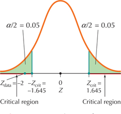FIGURE 5 Critical region for a two-tailed test.
Step 2 Find $Z_{crit}$ and state the rejection rule.

We have a two-tailed test and level of significance $α = 0.10$ . Using this information, Table 4 tells us that the critical value $Z_{crit} = 1.645$ and that we will reject $H_{0}$ if $Z_{data} \leq - 1.645$ or if $Z_{data} \geq 1.645$ (Figure 5).
Step 3 Calculate $Z_{data}$ .

We have $\bar{x} = 11.8$ , $n = 25$ , $σ = 5$ , and $μ_{0} = 13.8$ . Substituting:

$Z_{data} = \frac{\bar{x} - μ_{0}}{σ / \sqrt{n}} = \frac{11.8 - 13.8}{5 / \sqrt{25}} = - 2$
Step 4 State the conclusion and the interpretation.

$Z_{data} = - 2$ , which is ≤−1.645. Therefore we reject $H_{0}$ . There is evidence at level of significance $α = 0.10$ that the population mean hemoglobin level differs from 13.8 g/dl.

NOW YOU CAN DO

Exercises 45–48.

9.2 Z<math><mi>Z</mi></math> Test for the Population Mean: Critical-Value Method

9.2 $Z$ Test for the Population Mean: Critical-Value Method