9.3 Z Test for the Population Mean: p-Value Method
 This page includes Video Technology Manuals
 This page includes Statistical Videos
OBJECTIVES By the end of this section, I will be able to …
- Perform the Z test for the mean, using the p-value method.
- Assess the strength of evidence against the null hypothesis.
- Describe the relationship between the p-value method and the critical-value method.
- Use the Z confidence interval for the mean to perform the two-tailed Z test for the mean.
1 The p-Value Method of Performing the Z Test for the Mean
In Section 9.2, we considered the critical-value method for performing the Z test, which works by comparing one Z-value (Zdata) with another Z-value (Zcrit). In this section, we introduce the p-value method, which works by comparing one probability (the p-value) to another probability (α). The two methods are equivalent for the same level of significance α, giving you the same conclusion.
The p-value is a measure of how well (or how poorly) the data fit the null hypothesis.
p-Value
The p-value is the probability of observing a sample statistic (such as ˉx or Zdata) at least as extreme as the statistic actually observed if we assume that the null hypothesis is true.
Roughly speaking, the p-value represents the probability of observing the sample statistic if the null hypothesis is true. The term p-value means “probability value,” so its value must always lie between 0 and 1.
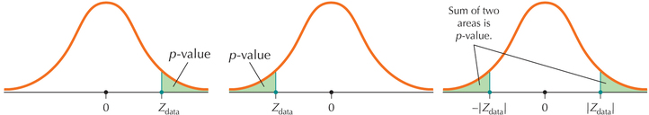
A p-value is a probability associated with Zdata and tells us whether or not Zdata is an extreme value. The method for calculating p-values depends on the form of the hypothesis test (Table 5).
- For a right-tailed test, the p-value is in the right (or upper) tail area.
- For a left-tailed test, the p-value is in the left (or lower) tail area.
- For a two-tailed test, the p-value lies in both tails.
Remember that probability is represented by the area under the curve.
| Type of hypothesis test | Right-tailed test | Left-tailed test | Two-tailed test |
|---|---|---|---|
| Hypotheses | H0:μ=μ0Ha:μ>μ0 | H0:μ=μ0Ha:μ<μ0 | H0:μ=μ0Ha:μ≠μ0 |
| p-Value is tail area associated with Zdata |
p-value=P(Z>Zdata) Area to right of Zdata |
p-value=P(Z<Zdata) Area to left of Zdata |
p-value=P(Z>|Zdata|)+P(Z<-|Zdata|)=2·P(Z>|Zdata|) Sum of the two tail areas |
|
|||
EXAMPLE 12 Finding the p-value
For each of the following hypothesis tests, calculate and graph the p-value.
- H0:μ=3.0 versus Ha:μ>3.0,Zdata=1
- H0:μ=10 versus Ha:μ<10,Zdata=-1.45
- H0:μ=100 versus Ha:μ≠100,Zdata=-2
To review how to calculate these probabilities, see Table 8 in Chapter 6 on page 355.
Solution
We have a right-tailed test, so that the p-value equals the area in the right tail:
p-value=P(Z>Zdata)=P(Z>1)
The Z table gives the probability for P(Z<1). Thus,
p-value=P(Z>1)=1-P(Z<1)=1-0.8413=0.1587 (Figure 6a)
We have a left-tailed test, so that the p-value equals the area in the left tail:
p-value=P(Z<Zdata)=P(Z<-1.45)=0.0735 (Figure 6b)
Page 509Here, we have a two-tailed test, so that the p-value equals the sum of the areas in the two tails:
p-value=P(Z>|Zdata|)+(Z<-|Zdata|)=P(Z>|- 2|)+(Z<-|- 2|)=P(Z>2)+(Z<-2)=0.0228+0.0228=0.0456 (Figure 6c)
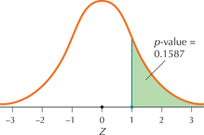 FIGURE 6a p-Value for a right-tailed test.
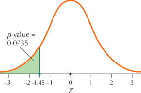 FIGURE 6b p-Value for a left-tailed test.
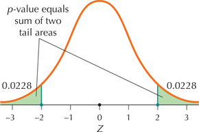 FIGURE 6c p-Value for a two-tailed test.
NOW YOU CAN DO
Exercises 7–20.
YOUR TURN#5
For each of the following hypothesis tests, calculate and graph the p-value.
- H0:μ=75 versus Ha:μ>75,Zdata=0.5
- H0:μ=50 versus Ha:μ<50,Zdata=-1.2
- H0:μ=1 versus Ha:μ≠1,Zdata=-0.1
(The solutions are shown in Appendix A.)
![]() The p-Value applet allows you to experiment with various hypotheses, means, standard deviations, and sample sizes in order to see how changes in these values affect the p-value.
The p-Value applet allows you to experiment with various hypotheses, means, standard deviations, and sample sizes in order to see how changes in these values affect the p-value.
A p-value is based on the value of Zdata, so the p-value tells us whether or not Zdata is an extreme value. Unusual and extreme values of ˉx, and therefore of Zdata, will have a small p-value, whereas values of ˉx and Zdata nearer to the center of the distribution will have a large p-value.
Assuming H0 is true:
| Unusual and extreme values of ˉx and Zdata | ↔ | Small p-value (close to 0; see Figure 6c) |
| Values of ˉx and Zdata near center | ↔ | Large p-value (greater than, say, 0.15; see Figure 6a) |
A small p-value indicates a conflict between your sample data and the null hypothesis, and will thus lead us to reject H0. However, how small is small? We learned in Section 9.1 that the probability of Type I error α is chosen by the researcher to be small, usually 0.01, 0.05, or 0.10. Thus, a p-value is small if it is ≤ α. This leads us to the rejection rule that tells us when we may reject the null hypothesis.
Rejection Rule When Using p-Value Method
The rejection rule for performing a hypothesis test using the p-value method is:
Reject H0 when the p-value ≤ α. Otherwise, do not reject H0.
This rejection rule can be applied to any type of hypothesis test we perform in Chapters 9–14 using the p-value method.
The value of α represents the boundary between results that are statistically significant (where we reject H0) and results that are not statistically significant (where we do not reject H0). Thus, α is called the level of significance of the hypothesis test.
Here are the steps for performing the Z test for μ using the p-value method.
Z Test for the Population Mean μ: p-Value Method
When a random sample of size n is taken from a population where the standard deviation σ is known, you can use the Z test if either (a) the population is normal, or (b) the sample size is large (n≥30).
Step 1 State the hypotheses and the rejection rule.
Use one of the forms from Table 5 to write the hypotheses. State the meaning of μ. The rejection rule is “Reject H0 if the p-value ≤ α.”
Step 2 Calculate Zdata.
Zdata=ˉx-μ0σ/√n
where the sample mean ˉx and the sample size n represent the sample data, and the population standard deviation σ represents the population data.
Step 3 Find the p-value.
Either use technology to find the p-value, or calculate it using the form in Table 5 that corresponds to your hypotheses.
Step 4 State the conclusion and interpretation.
If the p-value ≤ α, then reject H0. Otherwise do not reject H0. Interpret your conclusion so that a nonspecialist (someone who has not had a course in statistics) can understand, as follows:
- Interpretation when you reject H0: There is evidence at level of significance α that [whatever Ha says].
- Interpretation when you do not reject H0: There is insufficient evidence at level of significance α that [whatever Ha says].
EXAMPLE 13 The Z test for the mean using the p-value method: One-tailed test
FlightStats.com compiles user ratings for airports worldwide. The mean rating for JFK International Airport in New York for July 2014 was 3.0 (out of 5). Assume that the population standard deviation of user ratings is known to be σ=1. A random sample taken this year of n=36 user ratings for JFK Airport showed a mean of ˉx=2.75. Using level of significance α=0.05, test whether the population mean user rating for JFK Airport has fallen since 2014.
Solution
The sample size n=36 is large, and the population standard deviation σ is known. We may therefore perform the Z test for the mean.
Step 1 State the hypotheses and the rejection rule.
The key words here are “has fallen,” which means “is less than.” The answer to the question “Less than what?” gives us μ0=3.0. Thus, our hypotheses are
H0:μ=3.0 versus Ha:μ<3.0
where μ refers to the population mean user rating for JFK Airport. We will reject H0 if the p-value≤α=0.05.
Step 2 Calculate Zdata.
We have ˉx=2.75,μ0=3.0,n=36,, and σ=1. Thus, our test statistic is
Zdata=ˉx-μ0σ/√n=2.75-3.01/√36=-1.5
Page 511Step 3 Find the p-value.
Our hypotheses represent a left-tailed test from Table 5. Thus,
p-value=P(Z<Zdata)=P(Z<-1.5)
This is a Case 1 problem from Table 8 in Chapter 6 (page 355). The Z table (Appendix Table C) provides us with the area to the left of Z=-1.5 (Figure 7):
P(Z<-1.5)=0.0668
Thus, the p-value is 0.0668.
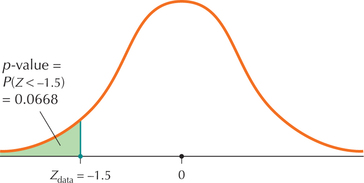 FIGURE 7 The p-value 0.0668 is not ≤ 0.05, so do not reject H0.
Step 4 State the conclusion and interpretation.
Our level of significance is α=0.05 (from Step 1). The p-value=0.0668 is not ≤ 0.05, therefore, we do not reject H0. There is insufficient evidence at the level of significance α=0.05 that the population mean user rating for JFK Airport is less than 3.0.
NOW YOU CAN DO
Exercises 21–26.
 What If Scenario
What if the sample mean in Example 13 was not ˉx=2.75 but was instead some unknown value smaller than ˉx=2.75? All other statistics and parameters remain the same. Suppose we wanted to perform the same hypothesis test as in Example 13. How would this decrease in the value of ˉx affect the following, if at all?
- Zdata
- p-value
- The conclusion
Solution
- In Example 13, ˉx=2.75 is smaller than μ0=3.0, which is why Zdata is negative. If we decrease ˉx to an even smaller value, this will move Zdata further into negative territory (leftward on the number line).
- For a left-tailed test, the p-value is the area to the left of Zdata. So, if Zdata is further to the left, there is less area to the left of it. Thus, the new p-value will be smaller.
- We know from (b) that the p-value is decreasing, but not by how much, because we don't know how much smaller ˉx and Zdata are. If the p-value decreases just a little bit, it will still be greater than α=0.05, and so we will still not reject H0. However, if the p-value decreases by a lot, it will then be less than α=0.05, and so then we will reject H0. Without further information, we just don't know.
EXAMPLE 14 The p-value method using technology: Two-tailed test
brisbane
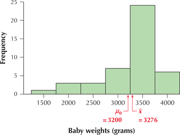
The birth weights, in grams (1000 grams = 1 kilogram ≈ 2.2 pounds), of a random sample of 44 babies from Brisbane, Australia, have a sample mean weight ˉx=3276 grams. Formerly, the mean birth weight of babies in Brisbane was 3200 grams. Assume that the population standard deviation σ=528 grams. Is there evidence that the population mean birth weight of Brisbane babies now differs from 3200 grams? Use technology to perform the appropriate hypothesis test, with level of significance α=0.10.
What Results Might We Expect?
Note from Figure 8 that the sample mean birth weight ˉx=3276 grams is close to the hypothesized mean birth weight of μ0=3200 grams. This value of ˉx is not extreme and thus does not seem to offer strong evidence that the hypothesized mean birth weight is wrong. Therefore, we might expect to not reject the hypothesis that μ0=3200 grams.
Solution
The sample size n=44 is large and σ=528 is known, so we may proceed with the Z test for μ.
Step 1 State the hypotheses and the rejection rule.
The key words “differs from” mean that we have a two-tailed test:
H0:μ=3200 versus Ha:μ≠3200
where μ refers to the population mean birth weight of Brisbane babies. We will reject H0 if the p-value≤α=0.10.
Step 2 Calculate Zdata.
We will use the instructions provided in the Step-by-Step Technology Guide at the end of this section (page 519). Figure 9 shows the TI-83/84 results from the Z test for μ:
FIGURE 9 TI-83/84 results.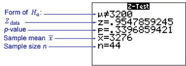 Page 513
Zdata=ˉx-μ0σ/√n=3276-3200528/√44=0.9547859245≈0.9548
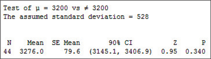
Figure 10 shows the Minitab results, where
- “Test of μ=3200 versus ≠ 3200” refers to the hypotheses being tested, H0:μ=3200 versus Ha:μ≠3200.
- “The assumed standard deviation = 528” refers to our assumption that σ=528.
- SE Mean refers to the standard error of the mean, that is, σ/√n. You can see that 528/√44≈79.6.
- 90% CI represents a 90% Z confidence interval for μ.
Z refers to our test statistic:
Zdata=ˉx-μ0σ/√n=(3276-3200)/(528/√44)=0.9547859245≈0.95
- P represents our p-value of 0.340.FIGURE 10 Minitab results.
Different software rounds the results to different numbers of decimal places.
Figure 11 shows the JMP results, where
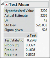
- “Hypothesized Value” refers to the hypotheses being tested: H0:μ=3200 versus Ha:μ≠3200.
- “Actual Estimate” refers to the sample mean, ˉx=3276.
- “Sigma given” refers to our assumption that σ=528.
- “Test statistic” refers to Zdata, our test statistic.
- “Prob>|z|,” “Prob>z,” and “Prob<z” refers to the p-value of a two-sided, right-tailed, and left-tailed test, respectively. We want the two-sided p-value, which is .
Step 3 Find the -value.
We have a two-tailed test from Step 1, so that from Table 5 our -value is (Figure 12)
FIGURE 12 -Value is the sum of two tail areas: .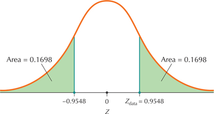 Page 514
Step 4 State the conclusion and interpretation.
Because 0.3396 is not ≤ 0.10, we do not reject . There is insufficient evidence that the population mean birth weight differs from 3200 grams. This conclusion is just as we expected.
NOW YOU CAN DO
Exercises 27–30.
2 Assessing the Strength of Evidence Against the Null Hypothesis
The hypothesis-testing methods we have shown so far deliver a simple “yes-or-no” conclusion: either “Reject ” or “Do not reject .” There is no indication of how strong the evidence is for rejecting the null hypothesis. Was the decision close? Was it a no-brainer? On the other hand, the -value itself represents the strength of evidence against the null hypothesis. There is extra information here, which we should not ignore.
For instance, we can directly compare the results of hypothesis tests. Suppose that we have two hypothesis tests that both result in not rejecting the null hypothesis, with level of significance . However, Test A has a -value of 0.06, whereas Test B has a -value of 0.57. Clearly, Test A came very close to rejecting the null hypothesis and shows a fair amount of evidence against the null hypothesis, whereas Test B shows no evidence at all against the null hypothesis. A simple statement of the “yes-or-no” conclusion misses the clear distinction between these two situations.
The -value provides us with the smallest level of significance at which the null hypothesis would be rejected, that is, the smallest value of at which the results would be considered significant.
Of course, we are free to determine whether the results are significant using whatever level we want. For example, Test A would have rejected for any value 0.06 or higher. Some data analysts in fact do not think in terms of rejecting or not rejecting the null hypothesis. Rather, they think completely in terms of assessing the strength of evidence against the null hypothesis.
For many (though not all) data domains, Table 6 provides a thumbnail impression of the strength of evidence against the null hypothesis for various -values. For certain domains (such as the physical sciences), however, alternative interpretations are appropriate.
| -Value | Strength of evidence against |
|---|---|
| Extremely strong evidence | |
| Very strong evidence | |
| Solid evidence | |
| Moderate evidence | |
| Slight evidence | |
| No evidence |
Note: Use Table 6 for all exercises that ask for an assessment of the strength of evidence against the null hypothesis.
EXAMPLE 15 Assessing the strength of evidence against
Assess the strength of evidence against shown by the -values in (a) Example 13 and (b) Example 14.
Solution
In Example 13, we tested versus , where refers to the population mean user rating for JFK International Airport. Our -value of 0.0668 implies that there is moderate evidence against the null hypothesis that the population mean user rating for JFK Airport equals 3.0.
Page 515- In Example 14, we tested versus , where refers to the population mean birth weight of Brisbane babies (in grams). Our -value of 0.3397 implies that there is no evidence against the null hypothesis that the population mean birth weight of Brisbane babies equals 3200 grams.
NOW YOU CAN DO
Exercises 31–40.
YOUR TURN#6
Each of the following -values was calculated in Example 12. For each, assess the strength of evidence against the null hypothesis.
(The solutions are shown in Appendix A.)
Developing Your Statistical Sense
The Role of the Level of Significance
Suppose that in Example 13, our level of significance was 0.10 instead of 0.05. Would this have changed anything? Certainly. Our -value of 0.0668 is less than the new , so we would reject . Think about that for a moment. The data haven't changed at all, but our conclusion is reversed simply by changing . What is a data analyst to make of a situation like this? Two alternatives are available.
- We don't want the choice of a to dictate our conclusion, so perhaps we should turn to a direct assessment of the strength of evidence against the null hypothesis, as provided in Table 6. In this case, the -value of about 0.0668 would offer moderate evidence against the null hypothesis, regardless of the value of .
- Obtain more data, perhaps through a call for further research.
3 The Relationship Between the -Value Method and the Critical-Value Method
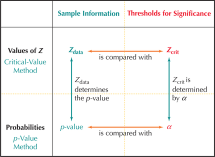
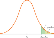
Figure 13 shows the relationships between the -value method and the critical-value method. The top half represents values of and the critical-value method that we studied in Section 9.2. The bottom half represents probabilities and the -value method that we studied in this section. The left half represents statistics associated with the observed sample data. The right half represents critical-value thresholds for significance to which these statistics are compared.
Because helps us to determine the -value, these two values are related. Similarly, because the level of significance helps to determine the value of , these two values are related. Moreover, just as we compare with the threshold , we compare the -value statistic with the threshold to determine significance. Thus, the two methods for conducting hypothesis tests are equivalent and, in fact, are quite thoroughly interwoven.
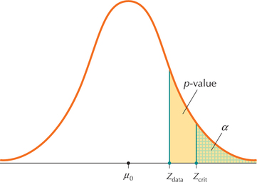
Figures 14a and 14b illustrate this equivalence for a right-tailed test. The rejection rule for the -value method is to reject when the . The rejection rule for the critical-value method is to reject when . Note in Figures 14a and 14b how the -value is determined by , and is determined by . In Figure 14a, when , it must also happen that the . In both cases we do not reject . However, in Figure 14b, when , it also follows that the . In both cases, we reject . Thus, the -value method and the critical-value method are equivalent.
4 Using Confidence Intervals for to Perform Two-Tailed Hypothesis Tests About
Consider a two-tailed hypothesis test for :
and recall the confidence interval for from Section 8.1:
Both inference methods are based on the statistic:
so it makes sense that the two-tailed hypothesis test and the confidence interval are equivalent.
Equivalence of a Two-Tailed Hypothesis Test and a Confidence Interval
- If a certain value for lies outside the corresponding confidence interval for , then the null hypothesis specifying this value for would be rejected for level of significance (see Figure 15).
- Alternatively, if a certain value for lies inside the confidence interval for , then the null hypothesis specifying this value for would not be rejected for level of significance .
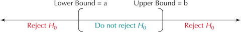
Table 7 shows the confidence levels and associated levels of significance that will produce the equivalent inference.
| Confidence level | Level of significance |
|---|---|
| 90% | 0.10 |
| 95% | 0.05 |
| 99% | 0.01 |
We may thus use a single confidence interval to test as many values of as necessary.
EXAMPLE 16 Equivalence of two-tailed tests and confidence intervals

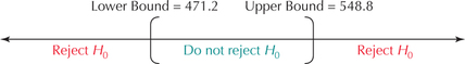
Recall Example 4 from Section 8.1 (page 432), where we were 90% confident using a interval that the population mean score on the 2014 SAT Math test lies between 471.2 and 548.8. Test, using level of significance , whether the population mean SAT Math test score differs from these values: (a) 470, (b) 510, (c) 550.
Solution
Once we have the 90% confidence interval, we may test as many possible values for as necessary, as long as we use level of significance (see Table 7).
- If any values of lie inside the confidence interval, that is, between 471.2 and 548.8, we will not reject for this value of .
- If any values of lie outside the confidence interval, that is, either to the left of 471.2 or to the right of 548.8, we will reject , as shown in Figure 16.FIGURE 16 Reject for values of that lie outside (471.2, 548.8).
We set up the three two-tailed hypothesis tests as follows:
To perform each hypothesis test, simply observe where each value of falls on the number line shown in Figure 16. For example, in the first hypothesis test, the hypothesized value lies outside the interval (471.2, 548.8). Thus, we reject . The three hypothesis tests are summarized here.
| Value of | Form of hypothesis test, with |
Where lies in relation to 90% confidence interval |
Conclusion of hypothesis test |
|---|---|---|---|
| a. 470 | Outside | Reject | |
| b. 510 | Inside | Do not reject | |
| c. 550 | Outside | Reject |
NOW YOU CAN DO
Exercises 41–46.
YOUR TURN#7
For the Z interval from Example 16, test, using level of significance , whether the population mean SAT Math test score differs from these values: (a) 548, (b) 477, (c) 549.
(The solutions are shown in Appendix A.)
Increasingly, technology is being used to perform statistical analysis, including hypothesis tests. Therefore, it is important to know how to read and interpret the software output from a hypothesis test.
EXAMPLE 17 Interpreting software output
Each of (a) and (b) represent software output from a Z test for . For each, examine the indicated software output, and provide the following steps:
- Step 1 State the hypotheses and the rejection rule.
- Step 2 Calculate .
- Step 3 Find the -value.
- Step 4 State the conclusion and interpretation.
Let the level of significance be in each case.
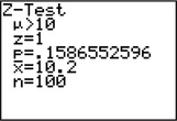
- TI-83/84 output for a Z test for , where represents the population mean length of laboratory mice (in cm)
- Minitab output for a test for , where represents the population mean number of farmer's markets per county, nationwide.
 TI-83/84 output for part (a).
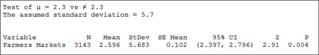 Minitab output for part (b).
Solution
Interpreting the TI-83/84 output.
Step 1 State the hypotheses and the rejection rule.
In the TI-83/84 output, the “” indicates the alternative hypothesis. In other words, the hypotheses are:
where represents the population mean length of laboratory mice (in cm). We will reject if the -value is less than the level of significance .
Page 519Step 2 Find .
The “” in the TI-83/84 output provides us the value of the test statistic, .
Step 3 Find the -value.
The “” in the TI-83/84 output represents the -value.
Step 4 State the conclusion and interpretation.
The -value from Step 3 is not less than the level of significance , so we do not reject . There is insufficient evidence that the population mean length of laboratory mice is greater than 10 cm.
- Interpreting the Minitab output.
Step 1 State the hypotheses and the rejection rule.
The first line in the Minitab output is “Test of ,” which indicates a two-tailed test, as follows:
where represents the population mean number of farmer's markets per county. We will reject if the -value is less than the level of significance .
Step 2 Find
Under “” in the Minitab output is found “2.91,” giving us .
Step 3 Find the -value.
Under “” in the Minitab output is “0.004,” representing our -value.
Step 4 State the conclusion and interpretation.
The -value (0.004) from Step 3 is less than the level of significance , so we reject .There is evidence that the population mean number of farmer's markets per county, nationwide, differs from 2.3.