Section 9.2 Exercises
CLARIFYING THE CONCEPTS
Question 9.36
1. What is the essential idea about hypothesis testing for the mean? (p. 498)
9.2.1
When the observed value of ˉx is unusual or extreme in the sampling distribution of ˉx that assumes H0 is true, we should reject H0. Otherwise, we should not reject H0.
Question 9.37
2. What does Zdata represent? (p. 499)
Question 9.38
3. Explain what a test statistic is. (p. 499)
9.2.3
A statistic generated from a data set for the purpose of testing a statistical hypothesis
Question 9.39
4. Describe the difference between the critical region and the noncritical region. (p. 500)
Question 9.40
5. Clearly describe what Zcrit is. (p. 500)
9.2.5
The value of Z that separates the critical region from the noncritical region.
Question 9.41
6. Suppose we reject H0 for the hypothesis test H0:μ=5 versus Ha:μ<5. Provide the generic interpretation. (p. 502)
Question 9.42
7. How did the right-tailed test get its name? (p. 501)
9.2.7
The critical region for a right-tailed test lies in the right (upper) tail.
Question 9.43
8. True or false: The value of Zcrit does not depend at all on the sample data. (p. 500)
PRACTICING THE TECHNIQUES
 CHECK IT OUT!
| To do | Check out | Topic |
|---|---|---|
| Exercises 9–22 | Example 7 | Calculating Zdata |
| Exercises 23–36 | Example 8 | Finding Zcrit and the critical region |
| Exercises 37–40 | Example 9 | Right-tailed Z test for μ |
| Exercises 41–44 | Example 10 | Left-tailed Z test for μ |
| Exercises 45–48 | Example 11 | Two-tailed Z test for μ |
For Exercises 9–48, assume that the conditions for performing the Z test are met.
For Exercises 9–20, calculate Zdata.
Question 9.44
9. H0:μ=75 vs. Ha:μ>75, ˉx=79, σ=20, n=25
9.2.9
Zdata=1
Question 9.45
10. H0:μ=75 vs. Ha:μ>75,ˉx=81,σ=20,n=25
Question 9.46
11. Right-tailed test with μ0=50 and σ=10. A sample of size 100 has a mean of 51.
9.2.11
Zdata=1
Question 9.47
12. Right-tailed test with μ0=50 and σ=10. A sample of size 100 has a mean of 54.
Question 9.48
13. H0:μ=98.6 vs. Ha:μ<98.6,ˉx=98.35,σ=1,n=16
9.2.13
Zdata=−1
Question 9.49
14. H0:μ=98.6 vs. Ha:μ<98.6,ˉx=97.85,σ=1,n=16
Question 9.50
15. Left-tailed test with μ0=20 and σ=5. A sample of size 100 has a mean of 19.
9.2.15
Zdata=−2
Question 9.51
16. Left-tailed test with μ0=20 and σ=5. A sample of size 100 has a mean of 18.5.
Question 9.52
17. H0:μ=1000 vs. Ha:μ≠1000,ˉx=1005,σ=100,n=400
9.2.17
Zdata=1
Question 9.53
18. H0:μ=1000 vs. Ha:μ≠1000,ˉx=995,σ=100,n=400
Question 9.54
19. Two-tailed test with μ0=2.5 and σ=0.5. A sample of size 100 has a mean of 2.45.
9.2.19
Zdata=−1
Question 9.55
20. Two-tailed test with μ0=2.5 and σ=0.5. A sample of size 100 has a mean of 2.55.
Question 9.56
21. Consider your results from Exercises 9–12. Describe what happens to Zdata for a right-tailed test as ˉx increases its distance above μ0, and everything else stays the same.
9.2.21
It increases.
Question 9.57
22. Consider your results from Exercises 13–16. Describe what happens to Zdata for a left-tailed test as ˉx increases its distance below μ0, and everything else stays the same.
For Exercises 23–34, do the following:
- Find the critical value Zcrit.
- Sketch the critical region, using the figures in Table 4 as a guide.
- State the rejection rule.
Question 9.58
23. H0:μ=75 vs. Ha:μ>75, level of significance α=0.10
9.2.23
(a) Zcrit=1.28
(b)
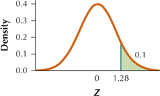
(c) Reject H0 if Zdata≥1.28.
Question 9.59
24. H0:μ=75 vs. Ha:μ>75, level of significance α=0.05
Question 9.60
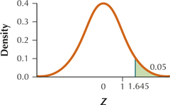
25. Right-tailed test with μ0=50, level of significance α=0.05
9.2.25
(a) Zcrit=1.645
(b)
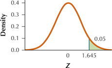
(c) Reject H0 if Zdata≥1.645.
Question 9.61
26. Right-tailed test with μ0=50, level of significance α=0.01
Question 9.62
27. H0:μ=98.6 vs. Ha:μ<98.6, level of significance α=0.05
9.2.27
(a) Zcrit=−1.645
(b)
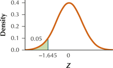
(c) Reject H0 if Zdata≤−1.645.
Question 9.63
28. H0:μ=98.6 vs. Ha:μ<98.6, level of significance α=0.01
Question 9.64
29. Left-tailed test with μ0=20, level of significance α=0.10
9.2.29
(a) Zcrit=−1.28
(b)
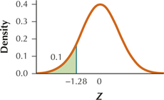
(c) Reject H0 if Zdata≤−1.28.
Question 9.65
30. Left-tailed test with μ0=20, level of significance α=0.05
Question 9.66
31. H0:μ=1000 vs. Ha:μ≠1000, level of significance α=0.05
9.2.31
(a) Zcrit=1.96
(b)
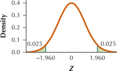
(c) Reject H0 if Zdata≤−1.96 or Zdata≥1.96.
Question 9.67
32. H0:μ=1000 vs. Ha:μ≠1000, level of significance α=0.01
Question 9.68
33. Two-tailed test with μ0=2.5, level of significance α=0.10
9.2.33
(a) Zcrit=1.645
(b)
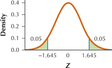
(c) Reject H0 if Zdata≤−1.645 or Zdata≥1.645.
Question 9.69
34. Two-tailed test with μ0=2.5, level of significance α=0.05
Question 9.70
35. Consider your results from Exercises 23–26. Describe what happens to (a) Zcrit and (b) the critical region, for a right-tailed test when the only change is the decrease in the level of significance α.
9.2.35
(a) Zcrit increases. (b) The critical region decreases.
Question 9.71
36. Consider your results from Exercises 27–30. Explain what happens to (a) Zcrit and (b) the critical region, for a left-tailed test as the level of significance a decreases but everything else stays the same.
For Exercises 37–48, use the hypotheses and data from the indicated exercises to perform the Z test for μ by doing the following steps:
- State the hypotheses.
- Find Zcrit and state the rejection rule.
- State the value of Zdata from the indicated exercise.
- State the conclusion and the interpretation.
Question 9.72
37. Use Zdata from Exercise 9 and Zcrit from Exercise 23.
9.2.37
(a) H0:μ=75 vs. Ha:μ>75 (b) Zcrit=1.28. Reject H0 if Zdata≥1.28.
(c) Zdata=1 (d) Zdata=1 is not ≥1.28. Therefore we do not reject H0. There is insufficient evidence at level of significance α=0.10 that the population mean is greater than 75.
Question 9.73
38. Use Zdata from Exercise 10 and Zcrit from Exercise 24.
Question 9.74
39. Use Zdata from Exercise 11 and Zcrit from Exercise 25.
9.2.39
(a) H0:μ=50 vs. Ha:μ>50 (b) Zcrit=1.645. Reject H0 if Zdata≥1.645. (c) Zdata=1 (d) Zdata=1 is not ≥1.645. Therefore we do not reject H0. There is insufficient evidence at level of significance α=0.05 that the population mean is greater than 50.
Question 9.75
40. Use Zdata from Exercise 12 and Zcrit from Exercise 26.
Question 9.76
41. Use Zdata from Exercise 13 and Zcrit from Exercise 27.
9.2.41
(a) H0:μ=98.6 vs. Ha:μ<98.6 (b) Zcrit=−1.645. Reject H0 if Zdata≤−1.645. (c) Zdata=−1 (d) Zdata=−1 is not ≤−1.645. Therefore we do not reject H0. There is insufficient evidence at level of significance α=0.05 that the population mean is less than 98.6.
Question 9.77
42. Use Zdata from Exercise 14 and Zcrit from Exercise 28.
Question 9.78
43. Use Zdata from Exercise 15 and Zcrit from Exercise 29.
9.2.43
(a) H0:μ=20 vs. Ha:μ<20 (b) Zcirt=−1.28. Reject H0 if Zdata≤−1.28. (c) Zdata=−2 (d) Zdata=−2 is ≤−1.28. Therefore we reject H0. There is evidence at level of significance α=0.10 that the population mean is less than 20.
Question 9.79
44. Use Zdata from Exercise 16 and Zcrit from Exercise 30.
Question 9.80
45. Use Zdata from Exercise 17 and Zcrit from Exercise 31.
9.2.45
(a) H0:μ=1000 vs. Ha:μ≠1000 (b) Zcrit=1.96. Reject H0 if Zdata≤−1.96 or Zdata≥1.96. (c) Zdata=1 (d) Zdata=1 is not ≤−1.96 and not ≥1.96. Therefore we do not reject H0. There is insufficient evidence at level of significance α=0.05 that the population mean differs from 1000.
Question 9.81
46. Use Zdata from Exercise 18 and Zcrit from Exercise 32.
Question 9.82
47. Use Zdata from Exercise 19 and Zcrit from Exercise 33
9.2.47
(a) H0:μ=2.5 vs. Ha:μ≠2.5 (b) Zcrit=1.645. Reject H0 if Zdata≤−1.645 orZdata≥1.645. (c) Zdata=−1 (d) Zdata=−1 is not ≤−1.645 and not ≥1.645. Therefore we do not reject H0. There is insufficient evidence at level of significance α=0.10 that the population mean differs from 2.5.
Question 9.83
48. Use Zdata from Exercise 20 and Zcrit from Exercise 34.
APPLYING THE CONCEPTS
For Exercises 49–56, do the following:
- State the hypotheses.
- Find Zcrit and the critical region.
- Find Zdata. Also, draw a standard normal Z curve showing Zcrit, the critical region, and Zdata.
- State the conclusion and the interpretation.
Question 9.84
49. Facebook Connections. According to Facebook.com, the mean number of community pages, groups, and events that users are connected to is 80. A random sample of 64 Facebook users showed a mean of 86 connections to community pages, groups, and events. Assume σ=48. Test, using level of significance α=0.05, whether the population mean number of connections to community pages, groups, and events is greater than 80.
9.2.49
(a) H0:μ=80 vs. Ha:μ>80 (b) Zcrit=1.645. Reject H0 if Zdata≥1.645. (c) Zdata=1.
(d) Since Zdata=1 is not ≥1.645, the conclusion is do not reject H0. There is insufficient evidence at the 0.05 level of significance that the population mean number of connections to community pages, groups, and events is greater than 80.
Question 9.85
50. Nurses' Study Time. The National Survey of Student Engagement reported that the mean number of hours spent studying per week for nursing majors is 18. Suppose a medical researcher obtained a random sample of 100 nursing majors, which yielded a sample mean study time of 19 hours. Assume σ=10 hours. Test, using level of significance α=0.05, whether the population mean study time for nursing majors is greater than 18 hours per week.
Question 9.86
51. Text Messages. The Pew Internet and American Life Project reports that young people ages 12–17 send a mean of 60 text messages per day. A random sample of 100 young people showed a mean of 69 text messages per day. Assume σ=30. Test, using level of significance α=0.01, whether the population mean number of text messages per day differs from 60.
9.2.51
(a) H0:μ=60 vs. Ha:μ≠60 (b) Zcrit=2.58. Reject H0 if Zdata≤−2.58 or Zdata≥2.58 (c) Zdata=3
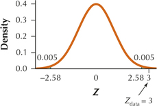
(d) Zdata=3 is ≥2.58. Therefore we reject H0. There is evidence at level of significance α=0.01 that the population mean number of text messages sent per day for young people ages 12–17 differs from 60.
Question 9.87
52. Video Gamers. Can't pry the PlayStation away from your dad? In 2015, the Entertainment Software Association reported that the mean age of video gamers was 35 years old. A recent random sample of 36 video gamers had a mean age of 34. Assume σ=6. Test, using level of significance α=0.05, whether the population mean age of video gamers is less than 35.
Question 9.88
53. Gas Prices. The American Automobile Association reported in June 2011 that the mean price for a gallon of regular gasoline was $3.70. A recent random sample of 25 gas stations had a mean price of $3.90. Assume normality and σ=$0.50. Test, using level of significance α=0.05, whether the population mean price for a gallon of regular gasoline has risen since June 2011.
9.2.53
(a) H0:μ=3.70 vs. Ha:μ>3.70 (b) Zcrit=1.645. Reject H0 if Zdata≥1.645. (c) Zdata=2.
(d) Since Zdata=2 is ≥1.645, the conclusion is reject H0. There is evidence at the 0.05 level of significance that the population mean price of regular gasoline is greater than $3.70 per gallon. Therefore we can conclude at the 0.05 level of significance that the population mean price for a gallon of regular gasoline has risen since June 2011.
Question 9.89
54. Online Shopping. The Nielsen organization reports that smartphone owners spent a mean of 93 minutes using shopping apps on their smartphones in the fourth quarter (last three months) of 2013. A random sample of 225 smartphone owners showed a mean of 99 minutes using shopping apps on their smartphones in the fourth quarter of last year. Assume σ=45 minutes. Conduct a hypothesis test, using level of significance α=0.10, to determine whether the population mean amount of time has changed.
Question 9.90
55. Americans' Height. A random sample of 400 American adults yields a mean height of 176 centimeters. Assume σ=2.5. Conduct a hypothesis test to investigate whether the population mean height of American adults has changed from 175 centimeters, using level of significance α=0.10.
9.2.55
(a) H0:μ=175 vs. Ha:μ≠175 (b) Zcrit=1.645. Reject H0 if Zdata≤−1.645 or if Zdata≥1.645. (c) Zdata=8.
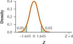
(d) Since Zdata=8 is ≥1.645, the conclusion is reject H0. There is evidence at the 0.10 level of significance that the population mean height of Americans has changed from 175 centimeters.
Question 9.91
56. Price of Milk. The U.S. Bureau of Labor Statistics reported that the mean price for a gallon of milk in 2011 was $3.34. A random sample of 100 retail establishments this year provides a mean price of $3.39. Assume σ=$0.25. Perform a hypothesis test, using level of significance α=0.05, to investigate whether the population mean price of milk this year has increased from the 2011 value.
Question 9.92
57. Automobile Operation Cost. The Bureau of Transportation Statistics reports that the mean cost of operating an automobile in the United States, including gas and oil, maintenance and tires, is 5.9 cents per mile. Suppose that a sample taken this year of 100 automobiles shows a mean operating cost of 6.2 cents per mile, and assume that the population standard deviation is 1.5 cents per mile. Test whether the population mean cost is greater than 5.9 cents per mile, using level of significance α=0.05.
- Is it appropriate to apply the Z test? Why or why not?
- We have a sample mean that is greater than the mean in the null hypothesis of 5.9 cents. Isn't this enough by itself to reject the null hypothesis? Explain why or why not.
- How many standard deviations above the mean is the 6.2 cents per mile? Do you think this is extreme?
9.2.57
(a) Since the sample size of n=100 is large (n≥30), Case 2 applies, so it is appropriate to apply the Z test. (b) Even though the sample mean ˉx=6.2 cents per mile is greater than the hypothesized mean μ=5.9 cents per mile, this is not enough by itself to reject the null hypothesis. It also depends on the variability of the data and on a0. (c) Since ˉx=6.2 cents per mile is 2 standard errors above μo=5.9 cents per mile, it is mildly extreme.
Question 9.93
58. Automobile Operation Cost. Refer to Exercise 57.
- Construct the hypotheses.
- Find the Z critical value and state the rejection rule.
- Calculate the value of the test statistic Zdata.
- State the conclusion and the interpretation.
Question 9.94
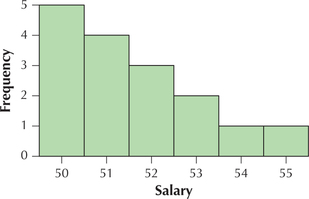
59. Accountants' Salaries. According to accountingWEB.com, the mean starting salary for a new accountant right out of college was $52,900 in 2014. A random sample of 16 new accountants has a mean salary of $54,000. We assume that the population standard deviation equals $4000. The histogram of the salary (in $1000s) is shown here. If it is appropriate to apply the Z test, then do so, using the critical-value method and level of significance α=0.05. If not, then explain clearly why not.
9.2.59
The histogram indicates that the data are extremely right-skewed and therefore not normally distributed. Thus Case 1 does not apply. Since the sample size of n=16 is small (n<30), Case 2 does not apply. Thus it is not appropriate to apply theZtest.
BRINGING IT ALL TOGETHER
Toyota Prius Gas Mileage. Use the following information for Exercises 60–67. Cars.com reported in 2014 that the mean city/highway combined gas mileage for the Toyota Prius hybrid car was 50 mpg. This year, a random sample of 16 Toyota Prius cars had the gas mileages shown here (in miles per gallon (mpg)). Assume σ=2 mpg. The research question is to test whether mean gas mileage has increased since 2014.
| 48.1 | 49.9 | 50.6 | 51.8 |
| 48.8 | 50.0 | 50.9 | 52.2 |
| 49.3 | 50.2 | 51.3 | 52.9 |
| 49.5 | 50.4 | 51.6 | 53.9 |
Question 9.95
60. Are the conditions met for performing the Z test for μ?
Use technology to obtain a normal probability plot of the data.
Question 9.96
61. Construct the appropriate hypotheses. State the meaning of μ.
9.2.61
H0:μ=50 vs. Ha:μ>50 where μ is the population mean city/highway combined gas mileage for the Toyota Prius hybrid car.
Question 9.97
62. Find the Z critical value and state the rejection rule. Use level of significance α=0.10.
Question 9.98
63. Calculate the value of Zdata.
9.2.63
Zdata=1.425.
Question 9.99
64. State and interpret your conclusion.
Question 9.100
 65. Try to answer the following questions by thinking about the relationship between the statistics instead of by redoing all the calculations. Note the mpg of the worst-performing Prius: 48.1. What if the 48.1 mpg is a typo? We are not sure what the actual mpg is, but it is greater than 48.1 mpg. How would this change affect the following?
- ˉx
- σ (Hint: This is not the sample standard deviation.)
- n
- Zdata
- Zcrit
- The conclusion
9.2.65
(a) Increase (b) Stay the same (c) Stay the same (d) Increase (e) Stay the same (f) Stay the same
Question 9.101
66. Now, instead of 0.10, use level of significance α=0.05. Find the new Z critical value and state the rejection rule.
There is no need to recalculate the value of Zdata. State and interpret your conclusion with this new level of significance α=0.05.
Question 9.102
67. Note the contradiction in your conclusions from Exercises 64 and 66. Can you suggest any way to resolve this?
9.2.67
Turn to a direct assessment of the strength of evidence against the null hypothesis or obtain more data.
WORKING WITH LARGE DATA SETS
Question 9.103
nutrition
68. Sodium. Work with the Nutrition data set.
- Use technology to explore the variable sodium.
- Use technology to test at level of significance α=0.05 whether the population mean amount of sodium is greater than 280 mg. Let σ=625 mg.
- Use technology to test at level of significance α=0.05 whether the population mean amount of sodium is greater than 290 mg. Let σ=625 mg.
WORKING WITH LARGE DATA SETS
 Chapter 9 Case Study: Clothing Store Sales. Open the Chapter 9 Case Study data set, Clothing Store. Here, we will perform a hypothesis test for the population mean number of coupons used per customer. We will then see whether this hypothesis test made the correct decision. Use technology to do the following.
Question 9.104
clothingstore
69. Obtain a random sample of size 100 from the data set.
Question 9.105
70. Using your sample, test whether the population mean number of coupons used per customer differs from 0.75, using level of significance α=0.05. Assume σ=1.74 coupons.
Question 9.106
71. Using the 5000 customers in the entire data set as a population, find the actual value of the population mean number of coupons used per customer. Did your hypothesis test in Exercise 71 make the right decision? Explain.
9.2.71
0.7724 coupon