18.5 The Modulation of Genetic Variation
What are the forces that modulate the amount of genetic variation in a population? How do new alleles enter the gene pool? What forces remove alleles from the gene pool? How can genetic variants be recombined to create novel combinations of alleles? Answers to these questions are at the heart of understanding the process of evolution. In this section, we will examine the roles of mutation, migration, recombination, genetic drift (chance), and selection in sculpting the genetic composition of populations.
New alleles enter the population: mutation and migration
Mutation is the ultimate source of all genetic variation. In Chapter 16, we discussed the molecular mechanisms that underlie small-
How can geneticists estimate the mutation rate? Geneticists can estimate mutation rates by starting with a single homozygous individual and following the pedigree of its descendants for several generations. Then they can compare the DNA sequence of the founding individual to the DNA sequences of the descendants several generations later and record any new mutations that have occurred. The number of observed mutations per genome per generation provides an estimate of the rate. Because one is looking for rather rare events, it is necessary to sequence billions of nucleotides to find just a few SNP mutations. In 2009, the SNP mutation rate for a part of the human Y chromosome was estimated by this approach to be 3.0 × 10⁻⁸ mutations/nucleotide/generation, or about one mutation every 30 million bp. If we extrapolate to the entire human genome (3 billion bp), then each of us has inherited 100 new mutations from each of our parents. Luckily, the vast majority of mutations are not detrimental since they occur in regions of the genome that are not critical.
Table 18-5 lists the mutation rates for SNPs and microsatellites in several model organisms. The SNP mutation rate is several orders of magnitude lower than the microsatellite rate. Their higher mutation rate and greater variation make microsatellites particularly useful in population genetics and DNA forensics. The SNP mutation rate per generation appears to be lower for unicellular organisms than for large multicellular organisms. This difference can be explained at least partially by the number of cell divisions per generation. There are about 200 cell divisions from zygote to gamete in humans but only 1 in E. coli. If the human rate is divided by 200, then the rate per cell division in humans is remarkably close to the rate in E. coli.
|
Organism |
SNP mutations (per bp) |
Microsatellite |
|---|---|---|
|
Arabidopsis |
7 × 10⁻⁹ |
9 × 10⁻⁴ |
|
Maize |
3 × 10⁻⁸ |
8 × 10⁻⁴ |
|
E. coli |
5 × 10⁻¹⁰ |
− |
|
Yeast |
5 × 10⁻¹⁰ |
4 × 10⁻⁵ |
|
C. elegans |
3 × 10⁻⁹ |
4 × 10⁻³ |
|
Drosophila |
4 × 10⁻⁹ |
9 × 10⁻⁶ |
|
Mouse |
4 × 10⁻⁹ |
3 × 10⁻⁴ |
|
Human |
3 × 10⁻⁸ |
6 × 10⁻⁴ |
|
Note: Microsatellite rate is for di- Source: Data from multiple published studies. |
||
Other than mutation, the only other means for new variation to enter a population is through migration or gene flow, the movement of individuals (or gametes) between populations. Most species are divided into a set of small local populations or subpopulations. Physical barriers such as oceans, rivers, or mountains may reduce gene flow between subpopulations, but often some degree of gene flow occurs despite such barriers. Within subpopulations, an individual may have a chance to mate with any other member of the opposite sex; however, individuals from different subpopulations cannot mate unless there is migration.
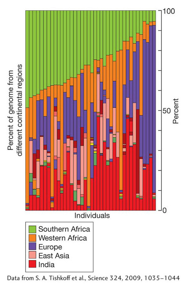
Isolated subpopulations tend to diverge as each accumulates its own unique mutations. Gene flow limits genetic divergence between subpopulations. One of the genetic consequences of migration is genetic admixture, the mix of genes that results when individuals have ancestry from more than one subpopulation. This phenomenon is common in human populations. It is readily observed in South Africa, where migrants from around the world were brought together. As shown in Figure 18-16, the genomes of South Africans of mixed ancestry are complex and include parts from the indigenous people of southern Africa plus contributions of migrants from western Africa, Europe, India, East Asia, and other regions.
KEY CONCEPT
Mutation is the ultimate source of all genetic variation. Migration can add genetic variation to a population via gene flow from another population of the same species.Recombination and linkage disequilibrium
Recombination is a critical force sculpting patterns of genetic variation in populations. In this case, alleles are not gained or lost; rather, recombination creates new haplotypes. Let’s look at how this works. Consider linked loci A and B. There could be a population in which only two haplotypes are found at generation t0: AB and ab. Suppose an individual in this population is heterozygous for these two haplotypes:

If a crossover occurs in this individual, then gametes with two new haplotypes, Ab and aB, could be formed and enter the population in generation t1.

Thus, recombination can create variation that takes the form of new haplotypes. The new haplotypes can have unique properties that alter protein function. For example, suppose an amino acid variant in a protein on one haplotype increases the enzyme activity of the protein twofold and a second amino acid variant on another haplotype also increases activity twofold. A recombination event that combines these two variants would yield a protein with fourfold higher activity.
Let’s now consider the observed and expected frequencies of the four possible haplotypes for two loci, each with two alleles. Linked loci, A and B, have alleles A and a and B and b with frequencies pA, pa, pB, and pb, respectively. The four possible haplotypes are AB, Ab, aB, and ab with observed frequencies PAB, PAb, PaB, and Pab. At what frequency do we expect to find each of these four haplotypes? If there is a random relationship between the alleles at the two loci, then the frequency of any haplotype will be the product of the frequencies of the two alleles that compose that haplotype:

For example, suppose that the frequency of each of the alleles is 0.5; that is, pA = pa = pB = pb = 0.5. When we sample the gene pool, the probability of drawing a chromosome with an A allele is 0.5. If the relationship between the alleles at locus A and the alleles at locus B is random, then the probability that the selected chromosome has the B allele is also 0.5. Thus, the probability that we draw a chromosome with the AB haplotype is

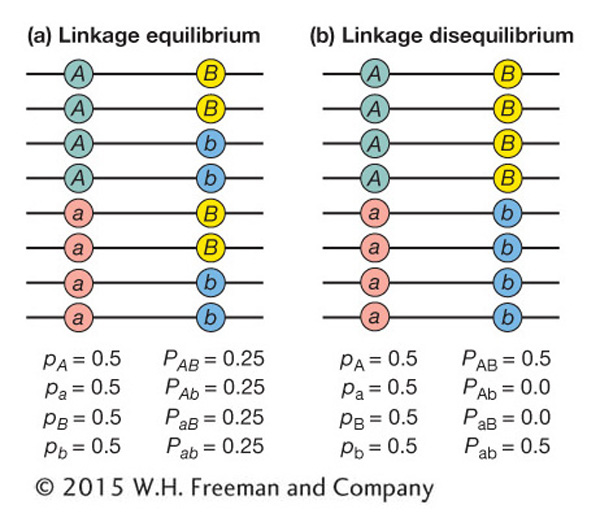
If the association between the alleles at two loci is random as just described, then the two loci are said to be at linkage equilibrium. In this case, the observed and expected frequencies will be the same. Figure 18-17a diagrams a case of two loci at linkage equilibrium.
If the association between the alleles at two loci is nonrandom, then the loci are said to be in linkage disequilibrium (LD). In this case, a specific allele at the first locus is associated with a specific allele at the second locus more often than expected by chance. Figure 18-17b diagrams a case of complete LD between two loci. The A allele is always associated with the B allele, while the a allele is always associated with the b allele. There are no chromosomes with haplotypes Ab or aB. In this case, the observed and expected frequencies will not be the same.
We can quantify the level of LD between two loci as the difference (D) between the observed frequency of a haplotype and the expected frequency given a random association among alleles at the two loci. If both loci involved have just two alleles, then

In Figure 18-17a, D = 0 since there is no LD, and in Figure 18-17b, D = 0.25, which is greater than 0, indicating the presence of LD.
How does LD arise? Whenever a new mutation occurs at a locus, the mutation appears on a single specific chromosome and so it is instantly linked to (or associated with) the specific alleles at any neighboring loci on that chromosome. Consider a population in which there are just two haplotypes: AB and Ab. If a new mutation (a) arises at the A locus on a chromosome that already possesses the b allele at the B locus, then a new ab haplotype would be formed. Over time, this new ab haplotype might rise in frequency in the population. Other chromosomes in the population would possess the AB or Ab haplotypes at these two loci, but no chromosomes would possess aB. Thus, the loci would be in LD. Migration can also cause LD when one subpopulation possesses only the AB haplotype and another only the ab haplotype. Any migrants between the subpopulations would give rise to LD within the subpopulation that receives the migrants.
LD between two loci will decline over time as crossovers between them randomize the relationship between their alleles. The rate of decline in LD depends on the rate at which crossing over occurs. The frequency of recombinants (RF) between the two loci among the gametes that form the next generation (see Chapter 4) provides an estimate of recombination rate, which in population genetics is symbolized by the lowercase letter r. If D0 is the value for linkage disequilibrium between two loci in the current generation, then the value in the next generation (D1) is given by this equation:

In other words, linkage disequilibrium as measured by D declines at a rate of (1 − r) per generation. When r is small, D declines slowly over time. When r is at its maximum (0.5), then D declines by 1/2 each generation.
Since LD decays as a function of time and the recombination fraction, population geneticists can use the level of LD between a mutation and the loci surrounding it to estimate the time in generations since the mutation first arose in the population. Older mutations have little LD with neighboring loci, while recent mutations show a high level of LD with neighboring loci. If you look again at Figure 18-14, you’ll notice that there is considerable LD between SNP2 in G6PD and the neighboring SNPs. SNP2 encodes the amino acid change of valine to methionine in the A− allele that confers resistance to malaria. Population geneticists have used LD at G6PD to estimate that the A− allele arose about 10,000 years ago. Malaria is not thought to have been prevalent in Africa until then. Thus, the A− arose by random mutation but was maintained in the population because it provided protection against malaria.
KEY CONCEPT
Linkage disequilibrium is the outcome of the fact that new mutations arise on a single haplotype. Linkage disequilibrium will decay over time because of recombination.Genetic drift and population size
The Hardy–
Let’s consider a simple but extreme case—
What happens if we increase the population size to N = 2 and the initial gene pool still has p = q = 0.5? The allele frequencies will change to p = 1 and q = 0 in the next generation only if the population consists of two A/A individuals. For this to happen, we need to draw four A alleles, each with a probability of p = 0.5, so the probability that the next generation will have p = 1 and q = 0.0 is p4 = (0.5)4 = 0.0625, or just over 6 percent. Thus, an N = 2 population is less likely to drift to fixation of the A allele than an N = 1 population. More generally, the probability of a population drifting to the fixation of the A allele in a single generation is p2N, and thus this probability gets progressively smaller as the population size (N) gets larger. Drift is a weaker force in large populations.
Drift means any change in allele frequencies due to sampling error, not just loss or fixation of an allele. In a population of N = 500 with two alleles at a frequency of p = q = 0.5, there are 500 copies of A and 500 copies of a. If the next generation has 501 copies of A (p = 0.501) and 499 copies of a (q = 0.499), then there has been genetic drift, albeit a very modest level of drift. A general formula for calculating the probability of observing a specific number of copies of an allele in the next generation, given the frequencies in the current generation, is presented in Box 18-
BOX 18-4 Allele Frequency Changes Under Drift
Consider a population of N diploid individuals segregating for two alleles A and a at the A locus with frequencies p and q, respectively. The population is random mating, and the size of the population remains the same (N) in each generation. When the gene pool is sampled to create the next generation, the exact number of copies of the A allele that are drawn cannot be strictly predicted because of sampling error. However, the probability that a specific number of copies of A will be drawn can be calculated using the binomial formula. Let k be a specific number of copies of the A allele. The probability of drawing k copies is

If we set N = 10 and p = q = 0.5, then the probability of drawing 10 copies of the A allele is

Thus, only 17.6 percent of the time will the next generation have the same frequency of A and a as the original generation. We can use this formula to calculate the outcomes for all possible values of k and obtain a probability distribution, shown in the figure below.
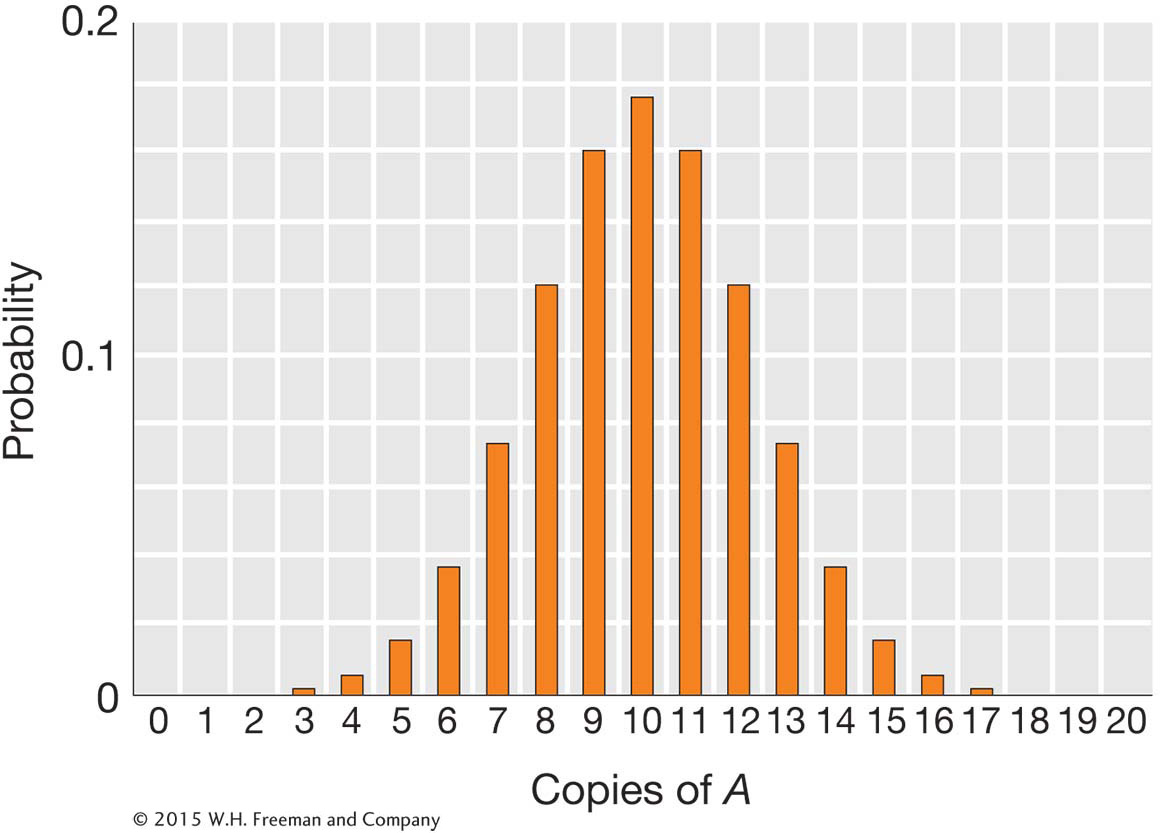
The most probable single outcome is no drift, with k = 10 and a probability of 0.176. However, the other outcomes all involve some drift, and so the probability that the population will experience some drift is 0.824.
When drift is operating in a finite population, one can calculate the probabilities of different outcomes, but one cannot accurately predict the specific outcome that will occur. The process is like rolling dice. At any locus, drift can continue from one generation to the next until one allele has become fixed. Also, in a particular population, the frequency of the A allele may increase from generation t0 to t1 but then decrease from generation t1 to t2. Drift does not proceed in a specific direction toward loss or fixation of an allele.
Figures 18-
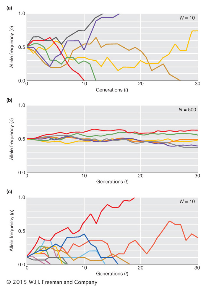
In addition to population size, the fate of an allele is determined by its frequency in the population. Specifically, the probability that an allele will drift to fixation in a future generation is equal to its frequency in the present generation. An allele that is at a frequency of 0.5 has a 50:50 chance of fixation or loss from the population in a future generation. You can see the effect of allele frequency on the fate of an allele in Figure 18-18c. For ten populations with an initial frequency of p = 0.1, eight populations experienced the loss of the A allele, one its fixation, and one population retained both alleles after 30 generations. That’s very close to the expectation that A will go to fixation 10 percent of the time when p = 0.1.
The fact that the frequency of an allele is equal to its probability of fixation means that most newly arising mutations will ultimately be lost from a population because of drift. The initial frequency of a new mutation in the gene pool is

If N is even modestly large, such as 10,000, then the probability that a new mutation will ultimately reach fixation is extremely small: 1/2N = 1/20,000 = 5 × 10⁻⁵. The probability that a new mutation will ultimately be lost from the population is

which is close to 1.0 in large populations. It is 0.99995 in a population of 10,000.
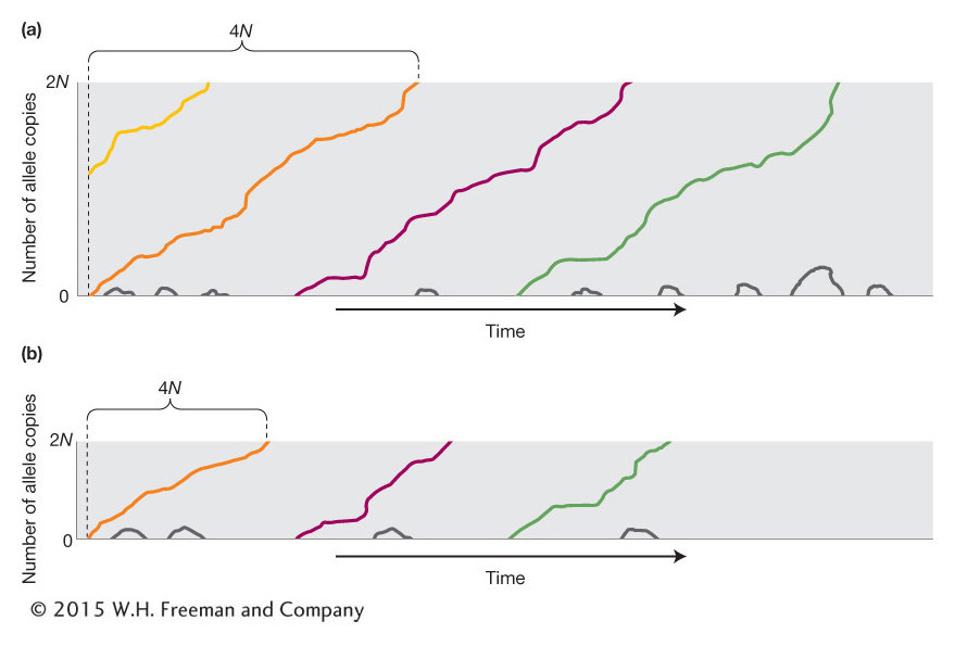
Figure 18-19a shows a graphical representation of the fate of new mutations in a population. The x-axis represents time and the y-axis the number of copies of an allele. The black lines show the fate of most new mutations. They appear and then are soon lost from the population. The colored lines show the few “lucky” new mutations that become fixed. From population genetic theory, it can be shown that the average time required for a lucky mutation to become fixed is 4N generations. Figure 18-19b shows a population that is 1/2 the size of the population in Figure 18-19a. Thus, 4N generations is 1/2 as long and the lucky new mutations are fixed more rapidly.
An important consequence of drift is that slightly deleterious alleles can be brought to fixation or advantageous alleles lost by this random process. Consider a new allele that arises in a population and endows the individual carrying it with a stronger immune system. This individual can pass the advantageous allele to his or her offspring, but those offspring might die before reproducing because of a random event such as being struck by lightning. Or if the individual carrying the favorable allele is heterozygous, he or she may pass only the less favorable allele to his or her offspring by chance.
In calculating the probabilities of different outcomes under genetic drift, we are assuming that the A and a alleles do not confer differences in viability or reproductive success to the individuals that carry them. We assume that A/A, A/a, and a/a individuals are all equally likely to survive and reproduce. In this case, A and a would be termed neutral alleles (or variants) relative to each other. Change in the frequencies of neutral alleles over time due to drift is called neutral evolution. The process of neutral evolution is the foundation for the molecular clock, the constant rate of substitution of newly arising allelic variants for preexisting ones over long periods (Box 18-
BOX 18-5 The Molecular Clock
As species diverge over time, their DNA sequences become increasingly different as mutations arise and become fixed in the population. At what rate do sequences diverge? To answer this question, consider a population at generation t0. The number of mutations that will appear in generation t1 is the product of the number of copies of the sequence in the gene pool (2N) times the rate at which they mutate (μ); that is, 2Nμ. If a mutation is neutral, then the probability that it drifts to fixation is 1/2N So each generation, 2Nμ new mutations enter the gene pool, and 1/2N of these will become fixed. The product of these two numbers is the rate (k) at which sequences evolve:

The value k is called the substitution rate, and it is equal to the mutation rate for neutral mutations. If the mutation rate remains constant over time, then the substitution rate will “tick” regularly like a clock, the molecular clock.
Consider two species A and B and their common ancestor. Let’s define d (divergence) as the number of neutral substitutions at nucleotide sites in the DNA sequence of a gene that have occurred since the divergence of A and B from their ancestor.
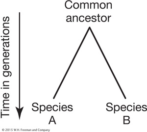
The expected value for d will be the product of the rate (k) at which substitutions occur and two times the time in generations (2t) during which substitution accumulated. The 2 is required because there are two lineages leading away from the common ancestor. Thus, we have

This equation can be rewritten as

showing how we can calculate the time in generations since the divergence of two species if we know d and k. The SNP mutation rate per generation (μ) is known for many groups of organisms (see Table 18-5), and it is the same as the substitution rate (k) for neutral mutations. One can sequence one or more genes from two species and determine the proportion of silent (neutral) nucleotide sites at which they differ and use this proportion as an estimate for d. Thus, one can calculate the time since two sequences (two species) diverged using the molecular clock. Between humans and chimps, there are about 0.018 base differences at synonymous sites in coding sequences. The SNP mutation rate for humans is 3 × 10⁻⁸, and the generation time is about 20 years. Using these values and the equation above, the estimated divergence time for humans and chimps is 6.0 million years ago. These calculations assume that the substitutions are neutral and that the rate of substitution has been constant over time.
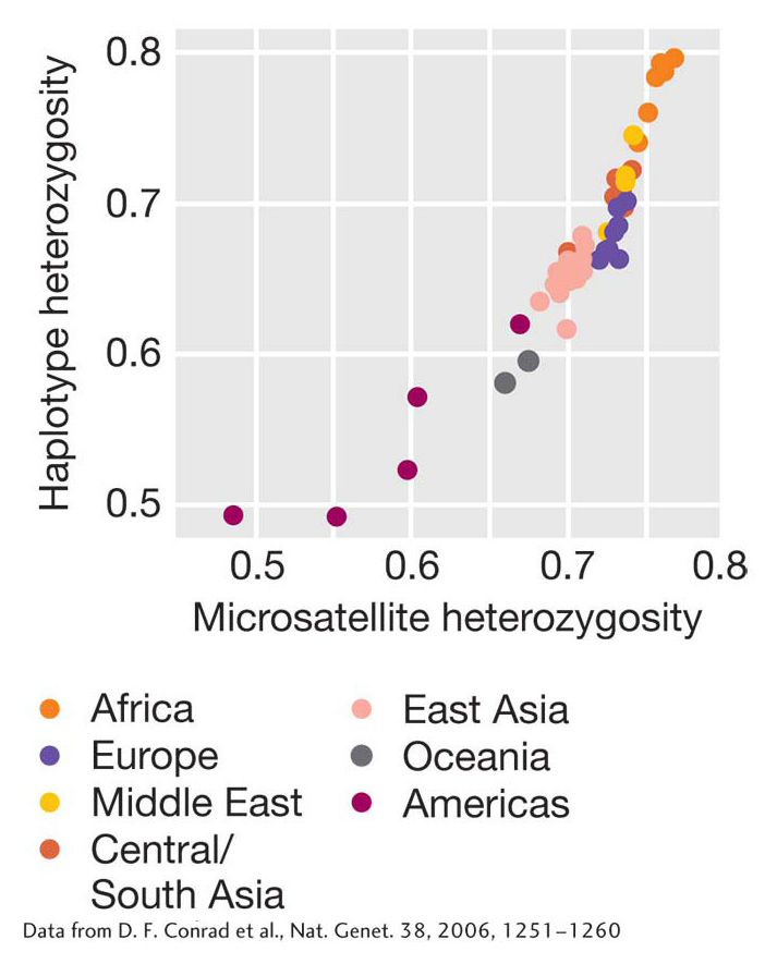
Up until now, we have been considering drift in the context of populations that remain the same size from one generation to the next. In reality, populations often contract or expand in size over time. For example, a new population of much smaller size can suddenly form when a relatively small number of the members of a population migrate to a new location and establish a new population. The migrants, or “founders,” of the new population may not carry all the alleles present in the original population, or they may carry the same alleles but at different frequencies. Genetic drift caused by random sampling of the original population to create the new population is known as the founder effect. One of many founder events in human history occurred when people crossed the Bering land bridge from Asia to the Americas during the ice age about 15,000 to 30,000 years ago. As a result, genetic diversity among Native Americans is lower than among people in other regions of the world (Figure 18-20).
Population size can also change within a single location. A period of one or several consecutive generations of contraction in population size is known as a population bottleneck. Bottlenecks occur in natural populations because of environmental fluctuations such as a reduction in the food supply or increase in predation. The gray wolf, American bison, bald eagle, California condor, whooping crane, and many whale species are some familiar examples of species that have experienced recent bottlenecks because of hunting by humans or encroachment by humans on their habitat. The reduction in population size during a bottleneck increases the level of drift in a population. As explained earlier in the chapter, the level of inbreeding in populations is also dependent on population size. Thus, bottlenecks also cause an increase in the level of inbreeding.
The California condor presents a remarkable example of a bottleneck. This species was once wide ranging but in the 1980s declined to a breeding population of only 14 captive birds. The population is now above 400 individuals, but the average heterozygosity in the genome decreased by 8 percent during the initial bottleneck. Furthermore, a deleterious recessive allele for a lethal form of dwarfism occurs at a frequency of about 9 percent among the surviving animals, presumably as a result of drift from a lower frequency in the pre-
Box 18-
BOX 18-6 The Domestication Bottleneck
Before 10,000 years ago, our ancestors around the world provided for themselves by hunting wild animals and collecting wild plant foods. At about that time, human societies began to develop farming. People took local wild plants and animals and bred them into crop plants and domesticated animals. Some of the major crops that were domesticated at this time include wheat in the Middle East, rice in Asia, sorghum in Africa, and maize in Mexico.
When the first farmers collected seeds from the wild to begin domestication, they drew a sample of the wild gene pool. This sample possessed only a subset of the genetic variation found in the wild. The domesticated populations were put through a bottleneck. As a consequence, crop plants and domesticated animals typically have less genetic variation than their wild progenitors.
Modern scientific plant breeding aimed at crop improvement has created a second bottleneck. By sampling the gene pool of the traditional crop varieties, modern plant breeders have created elite varieties with traits of commercial value such as high yield and suitability for mechanical harvesting and processing. As a consequence, elite or modern varieties have even less genetic variation than traditional varieties.
The loss of genetic variation resulting from the domestication and improvement bottlenecks can pose a threat. Since there are fewer alleles per locus, crops have a smaller repertoire of alleles at disease-
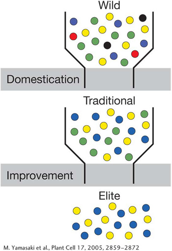
Crop domestication and improvement bottlenecks. Colored dots represent different alleles.
[M. Yamasaki et al., Plant Cell 17, 2005, 2859-
KEY CONCEPT
Population size is a key factor affecting genetic variation in populations. Genetic drift is a stronger force in small populations than in large ones. The probability that an allele will become fixed in (or lost from) a population by drift is a function of its frequency in the population and population size. Most new neutral mutations are lost from populations by drift.Selection
So far, we have considered how new alleles enter a population through mutation and migration and how these alleles can become fixed in (or lost from) a population by random drift. But mutation, migration, and drift cannot explain why organisms seem so well adapted to their environments. They cannot explain adaptations, features of an organism’s form or physiology that allow it to better cope with the environmental conditions under which it lives. To explain the origin of adaptations, Charles Darwin, in 1859 in his historic book The Origin of Species, proposed that adaptations arise through the action of another process, which he called “natural selection.” In this section, we will explore the role of natural selection in modulating genetic variation within populations. Later, in Chapter 20, we will consider the effects of natural selection on the evolution of genes and traits over extended periods.
Let’s define natural selection as the process by which individuals with certain heritable features are more likely to survive and reproduce than are other individuals that lack these features. As outlined by Darwin, the process works like this. In each generation more offspring are produced than can survive and reproduce in the environment. Nature has a mechanism (mutation) to generate new heritable forms or variants. Individuals with particular variants of some features are more likely to survive and reproduce. Individuals with features that enhance their ability to survive and reproduce will transmit these features to their offspring. Over time, these features will rise in frequency in the population. Thus, populations will change over time (evolve) as the environment (nature) favors (selects) features that enhance the ability to survive and reproduce. This is Darwin’s theory of evolution by means of natural selection.
Darwinian evolution is often described using the phrase “survival of the fittest.” This phrase can be misleading. An individual who is physically strong, resistant to disease, and lives a long life but has no offspring is not fit in the Darwinian sense. Darwinian fitness refers to the ability to survive and reproduce. It considers both viability and fecundity. One measure of Darwinian fitness is simply the number of offspring that an individual has. This measure is called absolute fitness, and we will symbolize it with an uppercase W. For an individual with no offspring, W equals 0, for an individual with one offspring, W equals 1, for an individual with two offspring, W equals 2, and so forth. W is also the number of alleles at a locus that an individual contributes to the gene pool.
Absolute fitness confounds population size and differences in reproductive success among individuals. Population geneticists are primarily interested in the latter, and so they use a measure called relative fitness (symbolized by a lowercase w), which is the fitness of an individual relative to some other individual, usually the most fit individual in the population. If individual X has two offspring and the most fit individual, Y, has 10 offspring, then the relative fitness of X is w = 2/10 = 0.2. The relative fitness of Y is w = 10/10 = 1. For every 10 alleles Y contributes to the next generation, X will contribute 2.
The concept of fitness applies to genotypes as well as to individuals. The absolute fitness for the A/A genotype (WA/A) is the average number of offspring left by individuals with that genotype. If we know the absolute fitnesses for all genotypes at a locus, we can calculate the relative fitnesses for each of the genotypes.
Let’s now look at how allele frequencies can change over time when different genotypes have different fitnesses; that is, when natural selection is at work. Below are the fitnesses and genotype frequencies for the three genotypes at the A locus in a population. In this case, A is a favored dominant allele since the fitnesses of the A/A and A/a individuals are the same and superior to the fitness of the a/a individuals. We are assuming that this population follows the Hardy–
|
A/A |
A/a |
a/a |
|
|
Average number of offspring (W) |
10 |
10 |
5 |
|
Relative fitness (w) |
1.0 |
1.0 |
0.5 |
|
Genotype frequency |
0.01 |
0.18 |
0.81 |
The relative contribution of each genotype to the gene pool is determined by the product of its fitness and its frequency. The more fit and the higher the frequency of a genotype, the more it contributes.
|
Genotype |
A/A |
A/a |
a/a |
Sum |
|---|---|---|---|---|
|
Relative contribution |
1 × 0.01 = 0.01 |
1 × 0.18 = 0.18 |
0.5 × 0.81 = 0.405 |
0.595 |
The relative contributions do not sum to 1, so we need to rescale them by dividing each by the sum of all three (0.595) to get the expected frequencies of the genotypes that contribute to the gene pool.
|
Genotype |
A/A |
A/a |
a/a |
Sum |
|---|---|---|---|---|
|
Genotype frequencies |
0.02 |
0.30 |
0.68 |
1.0 |
Using these expected genotype frequencies and the Hardy–

and

The difference between p′ and p (Δp = p′ − p) is 0.17 − 0.1 = 0.07, so we conclude that the A allele has climbed 7 percent in one generation due to natural selection. Box 18-
BOX 18-7 The Effect of Selection on Allele Frequencies
Selection causes change in allele frequencies between generations because some genotypes contribute more alleles to the gene pool than others. Let’s describe a set of equations to predict gene frequencies in the next generation when selection is operating. The genotype frequencies and absolute fitnesses are symbolized as follows:
|
genotype |
A/A |
A/a |
a/a |
|
frequency |
p2 |
2pq |
q2 |
|
absolute fitness |
WA/A |
WA/a |
Wa/a |
The average number of alleles contributed by individuals of a given genotype is the frequency of the genotype times the absolute fitness. If N is the population size, the total number of alleles contributed by all individuals of a given genotype is N multiplied by the average number of alleles contributed by individuals of a given genotype:
|
average number |
p2WA/A |
2pqWA/a |
q2Wa/a |
|
total number |
N(p2)Wa/a |
N(2pq)WA/a |
N(q2)Wa/a |
Thus, the gene pool will have

The mean fitness of the population is

which is the average number of alleles contributed to the gene pool by an individual. N is the total number of alleles in the gene pool.
We can now calculate the proportion of A alleles in the gene pool for the next generation as

This equation reduces to

Notice the expression pWA/A + qWA/a. This is called the allelic fitness or mean fitness of A alleles (WA):

From the Hardy–

This equation can be used calculate the frequency of A in the next generation and used recursively to follow the change in p over time.
Although we derived these formulas using absolute fitness, generally we are not interested in population size, so we use forms of these equations with relative fitness:

Finally, we can express change in allele frequency between generations as

But  , the mean relative fitness of the population, is the average of wA and wa, which are the allelic fitnesses of the A and a alleles, respectively:

Substituting this expression for  in the formula for Δp and remembering that q = 1 − p, we obtain

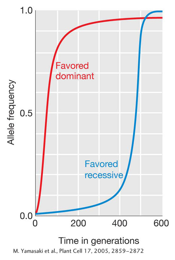
We could go through this process recursively, using the allele frequencies from the first generation to calculate those in the second generation, then using those from the second to calculate the third, and so forth. If we then plotted p by time measured in number of generations (t), we’d have a picture of the tempo with which allele frequencies change under the force of natural selection. Figure 18-21 shows such a plot for both a favored dominant and a favored recessive allele. The dominant allele rises rapidly to start but then hits a plateau and only slowly approaches fixation. Once the favored dominant allele is at a high frequency, the unfavored recessive allele occurs mostly in heterozygotes and rarely as homozygotes with reduced fitness, so selection is ineffective at purging it from the population. The favored recessive behaves in the opposite manner—
Forms of selection
Natural selection can operate in several different ways. Directional selection, which we have been discussing, moves the frequency of an allele in one direction until it reaches fixation or loss. Directional selection can be either positive or purifying. Positive selection works to bring a new, favorable mutation or allele to a higher frequency. This type of selection is at work when new adaptations evolve. A selective sweep occurs when a favorable allele reaches fixation. Directional selection can also work to remove deleterious mutations from the population. This form of selection is called purifying selection, and it prevents existing adaptive features from being degraded or lost. Selection does not always proceed directionally until loss or fixation of an allele. If the heterozygous class has a higher fitness than either of the homozygous classes, then natural selection will favor the maintenance of both alleles in the population. In this case, the locus is under balancing selection and natural selection will move the population to an equilibrium point at which both alleles are maintained in the population (see Chapter 20).
The different forms of selection each leave a distinct signature on the DNA sequence near the target locus in a population. For example, positive selection can be detected in DNA sequences by its effects on genetic diversity and linkage disequilibrium. Figure 18-22 shows schematic haplotypes before and after an episode of positive selection. In the panel showing the haplotypes before selection, the bracketed region has many polymorphisms and multiple haplotypes. However, after selection, there is only a single haplotype in this region and thus no polymorphism. When selection is applied to the target site (shown in red), the target and neighboring sites can all be swept to fixation before recombination breaks up the haplotype in which the favorable mutation first occurred. The result is lower diversity and higher LD near the target. As distance from the target increases, there is more opportunity for recombination, and so diversity goes gradually back up.
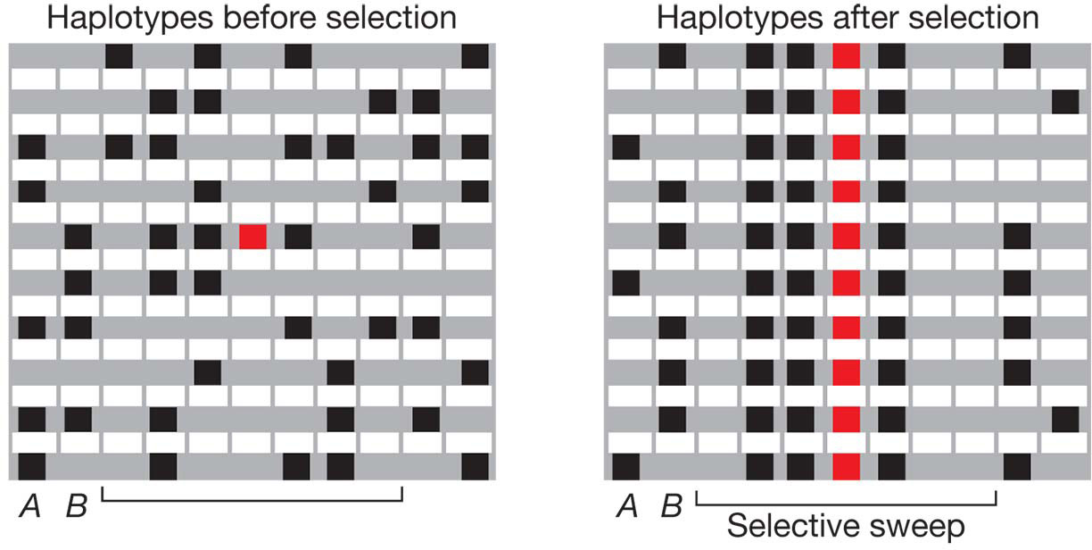
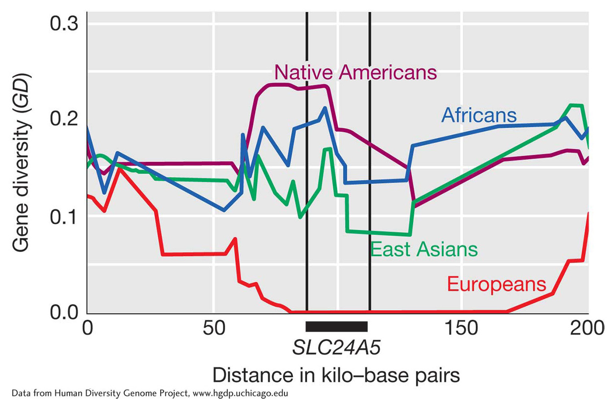
Figure 18-23 shows the pattern of diversity in the region surrounding the SLC24A5 gene in humans. This gene influences the deposition of the melanin in the skin. When people migrated from Africa to Europe, a selective sweep at SLC24A5 caused a loss of all diversity at this locus. As a consequence, there is a single allele and a single haplotype at this locus in Europe. The single allele that was selected for in Europe produces lighter skin color. Moving away from the gene in either direction, the number of haplotypes rises in European populations since recombination disrupted the linkage disequilibrium between SLC25A5 and more distance sites. Light skin may be adaptive in northern latitudes. People are able to synthesize vitamin D, but to do so they need to absorb UV radiation through the skin. In the equatorial latitudes, people are exposed to high levels of UV light and can synthesize vitamin D even with heavily pig-
Table 18-6 lists a few of the genes that show evidence for natural selection in modern humans. These genes fall into a few basic categories. One group strengthens resistance to pathogens. The genes G6PD, FYnull, and Hb (hemoglobin B, the sickle-
|
Gene |
Presumed Trait |
Population |
|---|---|---|
|
EDA2R (ectodysplasin A2 receptor) |
Male pattern baldness |
Europeans |
|
EDAR (ectodysplasin A receptor) |
Hair morphology |
East Asians |
|
FYnull (Duffy antigen) |
Resistance to malaria |
Africans |
|
G6PD (glucose- |
Resistance to malaria |
Africans |
|
Hb (hemoglobin B) |
Resistance to malaria |
Africans |
|
KITLG (KIT ligand) |
Skin pigmentation |
East Asians and Europeans |
|
LARGE (glycosyltransferase) |
Resistance to Lassa fever |
Africans |
|
LCT (lactase) |
Lactase persistence; ability to digest milk sugar as an adult |
Africans, Europeans |
|
LPR (leptin receptor) |
Processing of dietary fats |
East Asians |
|
MC1R (melanocortin receptor) |
Hair and skin pigmentation |
East Asians |
|
MHC (major histocompatibility complex) |
Infectious disease resistance |
Multiple populations |
|
OCA2 (oculocutaneous albinism) |
Skin pigmentation and eye color |
Europeans |
|
PPARD (peroxisome proliferator- |
Processing of dietary fats |
Europeans |
|
SI (sucrase- |
Sucrose metabolism |
East Asians |
|
SLC24A5 (solute carrier family 24) |
Skin pigmentation |
Europeans and West Asians |
|
TYRP1 (tyrosinase- |
Skin pigmentation |
Europeans |
|
Source: P. C. Sabeti et al., Science 312, 2006, 1614- |
||
Another group of selected genes in Table 18-6 adapts people to regional diets. Before 10,000 years ago, all humans were hunter–
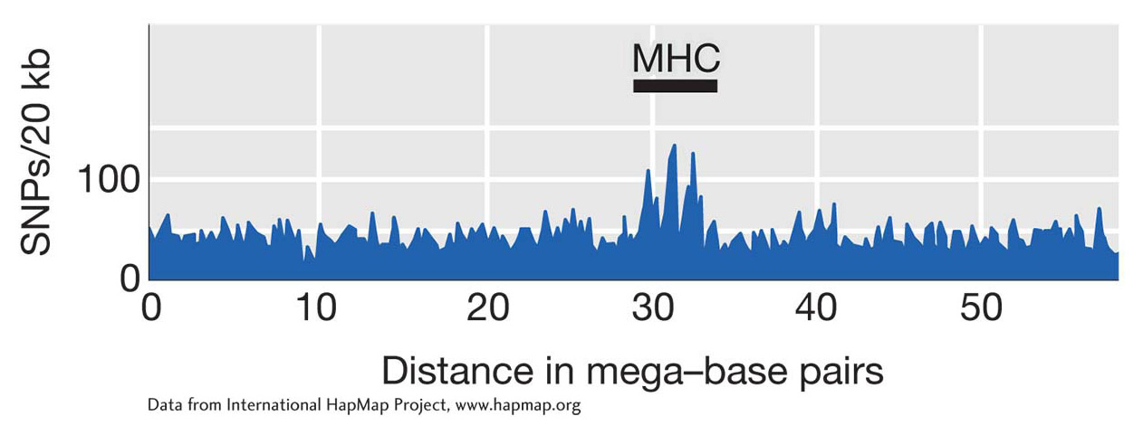
Whereas directional selection causes a loss of genetic variation in the region surrounding the target locus, balancing selection can prevent the loss of diversity by random genetic drift, leading to regions of unusually high genetic diversity in the genome. One region of high genetic diversity surrounds the major histocompatibility complex (MHC) gene complex on chromosome 6. Figure 18-24 shows a distinct spike in the number of SNPs at the MHC. This complex includes the human leukocyte antigen (HLA) genes, which are involved in immune system recognition of (and response to) pathogens. Balancing selection is one hypothesis proposed to explain the high diversity observed at the MHC. Since heterozygotes have two alleles, they may be resistant to a greater repertoire of pathogen types, giving heterozygotes a fitness advantage.
Finally, selection can be imposed by an agent other than nature. Humans have imposed selection in the process of domesticating and improving cultivated plants and animals. This form of selection is called artificial selection. In this case, individuals with traits that humans prefer contribute more alleles to the gene pool than individuals with unfavored traits. Over time, the alleles that confer the favored traits rise in frequency in the population. The many breeds of dogs and dairy cows and varieties of garden vegetables and cereal crops are all the products of artificial selection.
KEY CONCEPT
Natural selection is a force that can both drive favorable alleles at a locus to fixation or maintain multiple alleles at a locus in a population. Selection leaves a signature in the genome in the form of the pattern of genetic diversity surrounding the target of selection. Population geneticists have identified a number of genes that have been targets of selection in humans.Balance between mutation and drift
We have considered the forces that regulate variation in populations individually. Let’s now consider the opposing effects of mutation and drift, the former adding variation and the latter removing it from populations. When these two forces are in balance, a population can reach an equilibrium at which the loss and gain of variation are equal. We will use heterozygosity (H) as a measure of variation. Remember that H will be near 0 when a population is near fixation for a single allele (low variation), and H approaches 1 when there are many alleles of equal frequency (high variation).
Let’s use H with a “hat,”  , as the symbol for the equilibrium value of H. To find
  , we start with two mathematical equations: one equation that relates change in H to population size (drift) and another equation that relates change in H to the mutation rate. We can then set these equations equal to each other and solve for
  .
.
First, we need an equation for the decline in variation (H) between generations as a function of population size (drift). We developed such an equation in Box 18-

This equation applies to the effects of drift as well as those of inbreeding. From this equation, it follows that the change in H between generations due to drift is

Second, we need an equation for the increase in variation, as measured by H, between generations due to mutation. Any new mutation will increase heterozygosity at a rate proportional to the frequency of homozygotes in the population (1 − H) times the rate at which mutation converts them to heterozygotes (2μ). (The 2 is necessary because there are two alleles that could mutate in a diploid.) Thus, the change in H between generations due to mutation is

When the population reaches an equilibrium, the loss of heterozygosity by drift will be equal to the gain from mutation. Thus, we have

which can be rewritten as

This equation gives the equilibrium value of  when the loss by drift and gain by mutation are balanced. This equation applies only to neutral variation; that is, we are assuming selection is not at work. We are also assuming that each new mutation yields a unique allele.
Expressions such as this are useful when we have estimates for two of the variables and would like to know the third. For example, nucleotide diversity (H at the nucleotide level) for noncoding sequences, which are largely neutral, is about 0.0013 in humans, and μ for humans is 3 × 10⁻⁸ (see Table 18-5). Using these values and solving the equation above for N yields an estimate of the human population size of 10,498 humans. This estimate is far below the 7.2 billion of us alive today. What’s up? This is an estimate for the equilibrium value. Modern humans are a young group, only about 150,000 years old. Over the last 150,000 years, our population has grown dramatically as we filled the globe, but mutation is a slow process, so genetic diversity has not kept up and the human population is not at equilibrium. The population size of 10,498 represents an estimate of our historical size, or how many breeding members there were about 150,000 years ago.
Balance between mutation and selection
Allelic frequencies may also reach a stable equilibrium when the introduction of new alleles by repeated mutation is balanced by their removal by natural selection. This balance probably explains the persistence of genetic diseases as low-
Let’s begin with the simplest case—

Then, as shown in Box 18-

This equation shows that the frequency at equilibrium depends on the ratio μ/s. When the mutation rate for A → a gets larger and the selective disadvantage smaller, then the equilibrium frequency ( ) of a recessive deleterious allele will rise. As an example, a recessive lethal allele (s = 1) that arises by mutation from the wild-
Let’s consider the equilibrium between selection and mutation for the slightly more complicated case of a partially dominant deleterious allele—

where a is a partially dominant deleterious allele. A derivation similar to the one in Box 18-

BOX 18-8 The Balance Between Selection and Mutation
If we let q be the frequency of the deleterious allele a and p = 1 − q be the frequency of the normal allele A, then the change in allele frequency due to the mutation rate μ is

A simple way to express the fitnesses of the genotypes in the case of a recessive deleterious allele a is wA/A = wA/a = 1.0 and wa/a = 1 − s, where s, the selection coefficient, is the loss of fitness in the recessive homozygotes. We now can substitute these fitnesses in our general expression for allele frequency change (see Box 18-

Equilibrium means that the increase in the allele frequency due to mutation exactly balances the decrease in the allele frequency due to selection, so

The frequency of a recessive deleterious allele ( ) at equilibrium will be quite small, so
  , and we have

at equilibrium.
Here is an example. If μ = 10 6 and the lethal allele is not totally recessive but causes a 5 percent reduction in fitness in heterozygotes (s = 1.0, h = 0.05), then

This result is smaller by two orders of magnitude than the equilibrium frequency for the purely recessive case described above. In general, then, we can expect deleterious, completely recessive alleles to have frequencies much higher than those of partly dominant alleles because the recessive alleles are protected in heterozygotes.