6.1 The Production Function
A production function is the relationship between the quantity of inputs a firm uses and the quantity of output it produces.
A firm is an organization that produces goods or services for sale. To do this, it must transform inputs into output. The quantity of output a firm produces depends on the quantity of inputs; this relationship is known as the firm’s production function. As we’ll see, a firm’s production function underlies its cost curves. As a first step, let’s look at the characteristics of a hypothetical production function.
Inputs and Output
To understand the concept of a production function, let’s consider a farm that we assume, for the sake of simplicity, produces only one output, wheat, and uses only two inputs, land and labor. This particular farm is owned by a couple named George and Martha. They hire workers to do the actual physical labor on the farm. Moreover, we will assume that all potential workers are of the same quality—
A fixed input is an input whose quantity is fixed for a period of time and cannot be varied.
A variable input is an input whose quantity the firm can vary at any time.
George and Martha’s farm sits on 10 acres of land; no more acres are available to them, and they are currently unable to either increase or decrease the size of their farm by selling, buying, or leasing acreage. Land here is what economists call a fixed input—
The long run is the time period in which all inputs can be varied.
The short run is the time period in which at least one input is fixed.
In reality, whether or not the quantity of an input is really fixed depends on the time horizon. In the long run—
George and Martha know that the quantity of wheat they produce depends on the number of workers they hire. Using modern farming techniques, one worker can cultivate the 10-
The total product curve shows how the quantity of output depends on the quantity of the variable input, for a given quantity of the fixed input.
The relationship between the quantity of labor and the quantity of output, for a given amount of the fixed input, constitutes the farm’s production function. The production function for George and Martha’s farm, where land is the fixed input and labor is a variable input, is shown in the first two columns of the table in Figure 6-1; the diagram there shows the same information graphically. The curve in Figure 6-1 shows how the quantity of output depends on the quantity of the variable input, for a given quantity of the fixed input; it is called the farm’s total product curve.
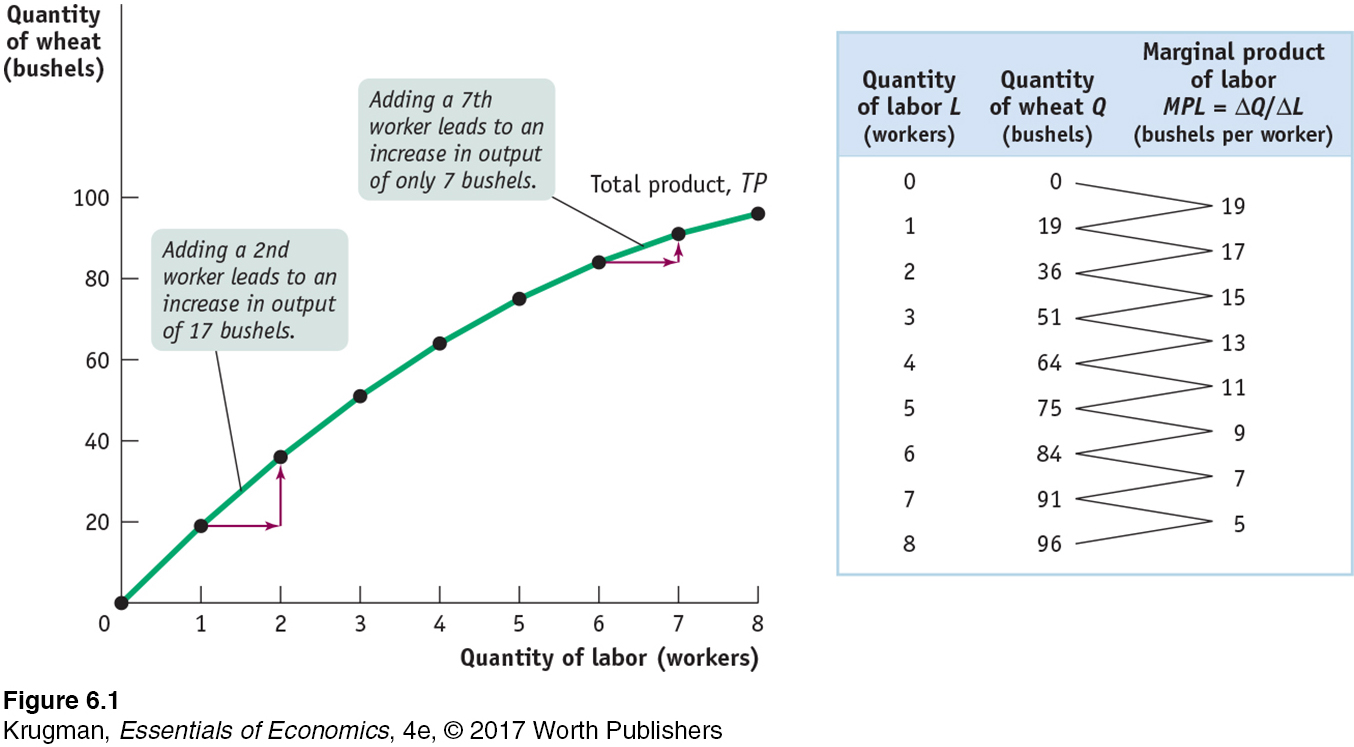
The physical quantity of output, bushels of wheat, is measured on the vertical axis; the quantity of the variable input, labor (that is, the number of workers employed), is measured on the horizontal axis. The total product curve here slopes upward, reflecting the fact that more bushels of wheat are produced as more workers are employed.
The marginal product of an input is the additional quantity of output that is produced by using one more unit of that input.
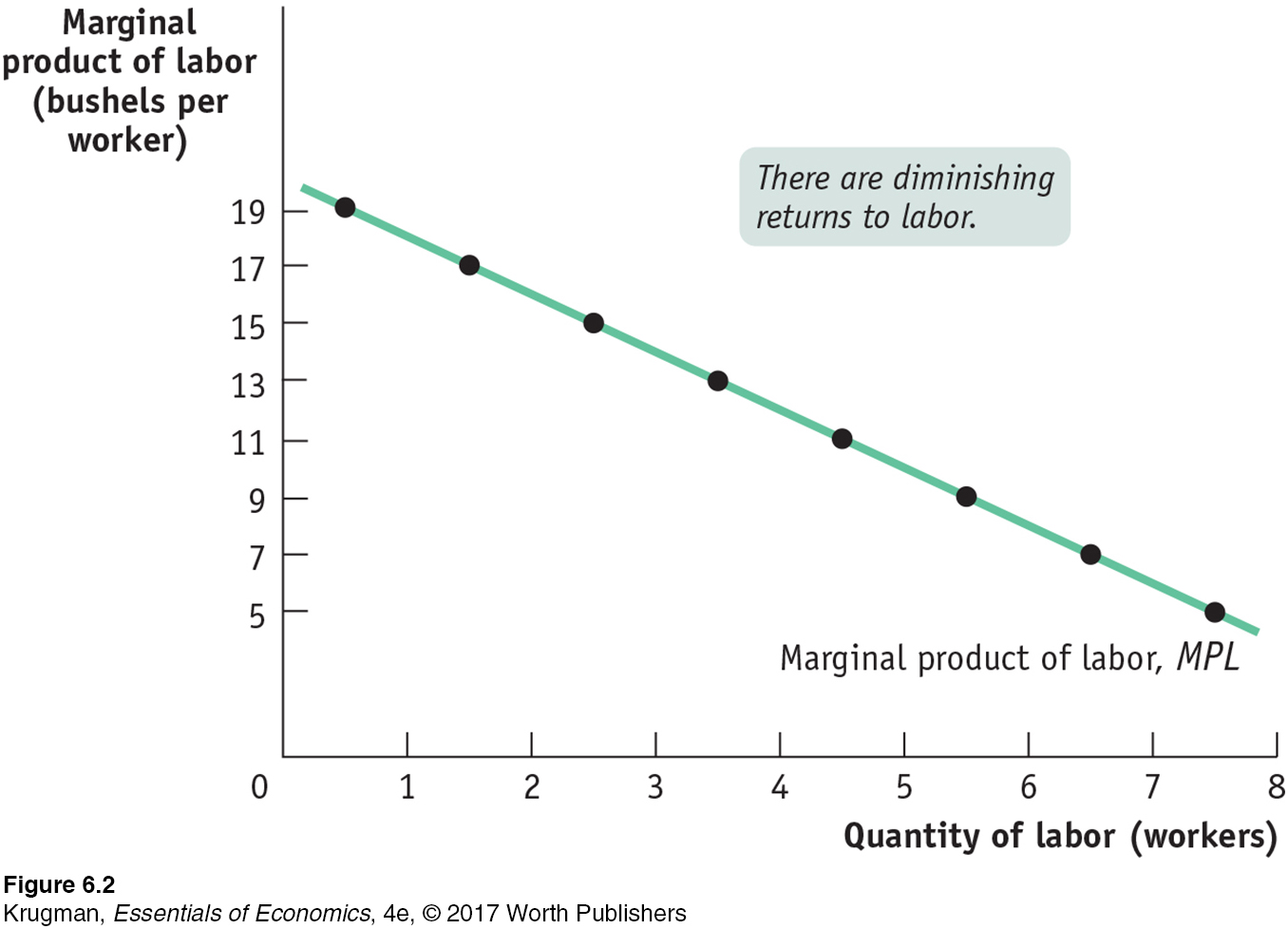
Although the total product curve in Figure 6-1 slopes upward along its entire length, the slope isn’t constant: as you move up the curve to the right, it flattens out. To understand why the slope changes, look at the third column of the table in Figure 6-1, which shows the change in the quantity of output that is generated by adding one more worker. This is called the marginal product of labor, or MPL: the additional quantity of output from using one more unit of labor (where one unit of labor is equal to one worker). In general, the marginal product of an input is the additional quantity of output that is produced by using one more unit of that input.
In this example, we have data on changes in output at intervals of 1 worker. Sometimes data aren’t available in increments of 1 unit—

or
In this equation, Δ, the Greek uppercase delta, represents the change in a variable.
![]() | interactive activity
| interactive activity
Now we can explain the significance of the slope of the total product curve: it is equal to the marginal product of labor. The slope of a line is equal to “rise” over “run” (see the appendix to Chapter 2). This implies that the slope of the total product curve is the change in the quantity of output (the “rise”, ΔQ) divided by the change in the quantity of labor (the “run”, ΔL). And this, as we can see from Equation 6-
GLOBAL
COMPARISON
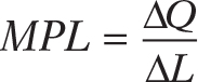
Wheat Yields Around the World
Wheat yields differ substantially around the world. The disparity between France and the United States that you see in this graph is particularly striking, given that they are both wealthy countries with comparable agricultural technology. Yet the reason for that disparity is straightforward: differing government policies. In the United States, farmers receive payments from the government to supplement their incomes, but European farmers benefit from price floors. Since European farmers get higher prices for their output than American farmers, they employ more variable inputs and produce significantly higher yields.
Interestingly, in poor countries like Uganda and Ethiopia, foreign aid can lead to significantly depressed yields. Foreign aid from wealthy countries has often taken the form of surplus food, which depresses local market prices, severely hurting the local agriculture that poor countries normally depend on. Charitable organizations like OXFAM have asked wealthy food-
Data from: Food and Agriculture Organization of the United Nations. Data are from 2012.
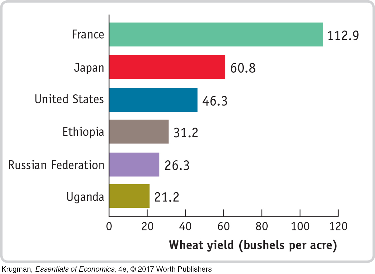
In this example, the marginal product of labor steadily declines as more workers are hired—
Figure 6-2 shows how the marginal product of labor depends on the number of workers employed on the farm. The marginal product of labor, MPL, is measured on the vertical axis in units of physical output—
There are diminishing returns to an input when an increase in the quantity of that input, holding the levels of all other inputs fixed, leads to a decline in the marginal product of that input.
In this example the marginal product of labor falls as the number of workers increases. That is, there are diminishing returns to labor on George and Martha’s farm. In general, there are diminishing returns to an input when an increase in the quantity of that input, holding the quantity of all other inputs fixed, reduces that input’s marginal product. Due to diminishing returns to labor, the MPL curve is negatively sloped.
To grasp why diminishing returns can occur, think about what happens as George and Martha add more and more workers without increasing the number of acres of land. As the number of workers increases, the land is farmed more intensively and the number of bushels produced increases. But each additional worker is working with a smaller share of the 10 acres—
The crucial point to emphasize about diminishing returns is that, like many propositions in economics, it is an “other things equal” proposition: each successive unit of an input will raise production by less than the last if the quantity of all other inputs is held fixed.
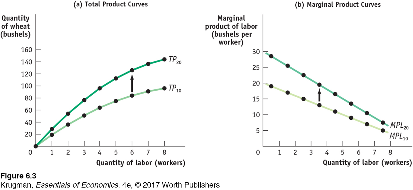
What would happen if the levels of other inputs were allowed to change? You can see the answer illustrated in Figure 6-3. Panel (a) shows two total product curves, TP10 and TP20. TP10 is the farm’s total product curve when its total area is 10 acres (the same curve as in Figure 6-1). TP20 is the total product curve when the farm has increased to 20 acres. Except when 0 workers are employed, TP20 lies everywhere above TP10 because with more acres available, any given number of workers produces more output. Panel (b) shows the corresponding marginal product of labor curves. MPL10 is the marginal product of labor curve given 10 acres to cultivate (the same curve as in Figure 6-2), and MPL20 is the marginal product of labor curve given 20 acres.
PITFALLS
WHAT’S A UNIT?
The marginal product of labor (or any other input) is defined as the increase in the quantity of output when you increase the quantity of that input by one unit. But what do we mean by a “unit” of labor? Is it an additional hour of labor, an additional week, or a person-
The answer is that it doesn’t matter, as long as you are consistent. One common source of error in economics is getting units confused—
Both curves slope downward because, in each case, the amount of land is fixed, albeit at different levels. But MPL20 lies everywhere above MPL10, reflecting the fact that the marginal product of the same worker is higher when he or she has more of the fixed input to work with.
Figure 6-3 demonstrates a general result: the position of the total product curve of a given input depends on the quantities of other inputs. If you change the quantity of the other inputs, both the total product curve and the marginal product curve of the remaining input will shift.
From the Production Function to Cost Curves
Once George and Martha know their production function, they know the relationship between inputs of labor and land and output of wheat. But if they want to maximize their profits, they need to translate this knowledge into information about the relationship between the quantity of output and cost. Let’s see how they can do this.
A fixed cost is a cost that does not depend on the quantity of output produced. It is the cost of the fixed input.
To translate information about a firm’s production function into information about its costs, we need to know how much the firm must pay for its inputs. We will assume that George and Martha face a cost of $400 for the use of the land. It is irrelevant whether George and Martha must rent 10 acres of the land for $400 from someone else or whether they own the land themselves and forgo earning $400 from renting it to someone else. Either way, they pay an opportunity cost of $400 by using the land to grow wheat. Moreover, since the land is a fixed input, the $400 George and Martha pay for it is a fixed cost, denoted by FC—a cost that does not depend on the quantity of output produced (in the short run). In business, fixed cost is often referred to as “overhead cost.”
A variable cost is a cost that depends on the quantity of output produced. It is the cost of the variable input.
The total cost of producing a given quantity of output is the sum of the fixed cost and the variable cost of producing that quantity of output.
We also assume that George and Martha must pay each worker $200. Using their production function, George and Martha know that the number of workers they must hire depends on the amount of wheat they intend to produce. So the cost of labor, which is equal to the number of workers multiplied by $200, is a variable cost, denoted by VC—a cost that depends on the quantity of output produced. It is variable because in order to produce more they have to employ more units of input. Adding the fixed cost and the variable cost of a given quantity of output gives the total cost, or TC, of that quantity of output. We can express the relationship among fixed cost, variable cost, and total cost as an equation:
(6-
or
TC = FC + VC
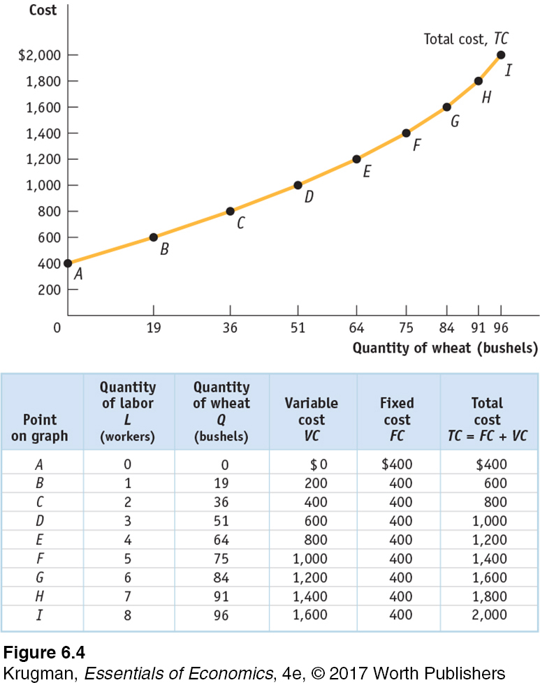
The table in Figure 6-4 shows how total cost is calculated for George and Martha’s farm. The second column shows the number of workers employed, L. The third column shows the corresponding level of output, Q, taken from the table in Figure 6-1. The fourth column shows the variable cost, VC, equal to the number of workers multiplied by $200, the cost per worker. The fifth column shows the fixed cost, FC, which is $400 regardless of how many workers are employed. The sixth column shows the total cost of output, TC, which is the variable cost plus the fixed cost.
The total cost curve shows how total cost depends on the quantity of output.
The first column labels each row of the table with a letter, from A to I. These labels will be helpful in understanding our next step: drawing the total cost curve, a curve that shows how total cost depends on the quantity of output.
George and Martha’s total cost curve is shown in the diagram in Figure 6-4, where the horizontal axis measures the quantity of output in bushels of wheat and the vertical axis measures total cost in dollars. Each point on the curve corresponds to one row of the table in Figure 6-4. For example, point A shows the situation when 0 workers are employed: output is 0, and total cost is equal to fixed cost, $400. Similarly, point B shows the situation when 1 worker is employed: output is 19 bushels, and total cost is $600, equal to the sum of $400 in fixed cost and $200 in variable cost.
Like the total product curve, the total cost curve slopes upward: due to the variable cost, the more output produced, the higher the farm’s total cost. But unlike the total product curve, which gets flatter as employment rises, the total cost curve gets steeper. That is, the slope of the total cost curve is greater as the amount of output produced increases. As we will soon see, the steepening of the total cost curve is also due to diminishing returns to the variable input. Before we can understand this, we must first look at the relationships among several useful measures of cost.
ECONOMICS in Action
The Mythical Man-
![]() | interactive activity
| interactive activity
The concept of diminishing returns to an input was first formulated by economists during the late eighteenth century. These economists, notably including Thomas Malthus, drew their inspiration from agricultural examples.
However, the idea of diminishing returns to an input applies with equal force to the most modern of economic activities—
The chapter that gave its title to the book is basically about diminishing returns to labor in the writing of software. Brooks observed that multiplying the number of programmers assigned to a project did not produce a proportionate reduction in the time it took to get the program written. A project that could be done by 1 programmer in 12 months could not be done by 12 programmers in 1 month—
The argument of The Mythical Man-
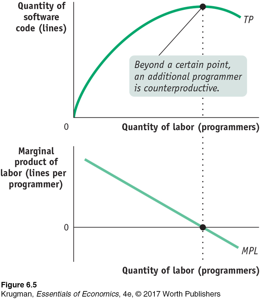
In other words, programming is subject to diminishing returns so severe that at some point more programmers actually have negative marginal product. The source of the diminishing returns lies in the nature of the production function for a programming project: each programmer must coordinate his or her work with that of all the other programmers on the project, leading each person to spend more time communicating with others as the number of programmers increases. In other words, other things equal, there are diminishing returns to labor. It is likely, however, that if fixed inputs devoted to programming projects are increased—
A reviewer of the reissued edition of The Mythical Man-
Quick Review
The firm’s production function is the relationship between quantity of inputs and quantity of output. The total product curve shows how the quantity of output depends on the quantity of the variable input for a given quantity of the fixed input, and its slope is equal to the marginal product of the variable input. In the short run, the fixed input cannot be varied; in the long run all inputs are variable.
When the levels of all other inputs are fixed, diminishing returns to an input may arise, yielding a downward-
sloping marginal product curve and a total product curve that becomes flatter as more output is produced. The total cost of a given quantity of output equals the fixed cost plus the variable cost of that output. The total cost curve becomes steeper as more output is produced due to diminishing returns to the variable input.
Check Your Understanding 6-1
Question 6.1
1. Bernie’s ice-
| Quantity of electricity (kilowatts) |
Quantity of ice (pounds) |
| 0 | 0 |
| 1 | 1,000 |
| 2 | 1,800 |
| 3 | 2,400 |
| 4 | 2,800 |
What is the fixed input? What is the variable input?
The fixed input is the 10-
ton machine, and the variable input is electricity. Construct a table showing the marginal product of the variable input. Does it show diminishing returns?
As you can see from the declining numbers in the third column of the accompanying table, electricity does indeed exhibit diminishing returns: the marginal product of each additional kilowatt of electricity is less than that of the previous kilowatt.
Quantity
of electricity
(kilowatts)Quantity of
ice (pounds)Marginal product
of electricity
(pounds per
kilowatt)0 0 1,000 1 1,000 800 2 1,800 600 3 2,400 400 4 2,800 Suppose a 50% increase in the size of the fixed input increases output by 100% for any given amount of the variable input. What is the fixed input now? Construct a table showing the quantity of output and marginal product in this case.
A 50% increase in the size of the fixed input means that Bernie now has a 15-
ton machine. So the fixed input is now the 15- ton machine. Since it generates a 100% increase in output for any given amount of electricity, the quantity of output and marginal product are now as shown in the accompanying table. Quantity of
electricity
(kilowatts)Quantity of ice
(pounds)Marginal product
of electricity
(pounds per
kilowatt)0 0 2,000 1 2,000 1,600 2 3,600 1,200 3 4,800 800 4 5,600