15.9 Stokes' TheoremPrinted Page 1045
ORIGINS
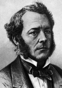
Stokes' Theorem is named after the Irish mathematician George Gabriel Stokes (1819–1903). Stokes, along with Maxwell and Kelvin, contributed to the prominence of the Cambridge School of Mathematical Physics.
Stokes' Theorem is a second generalization of Green's Theorem to space. Stokes' Theorem expresses a certain relationship between a line integral of a vector field F around a simple closed curve C in space to a surface integral for which C forms the boundary. The theorem is used in applications of electricity and magnetism, most notably in Ampere's Law and in the Maxwell–Faraday Law.
1046
To get started, we need the definition of the curl of F.
DEFINITION Curl of F
Let F=F(x,y,z)=P(x,y,z)i+Q(x,y,z)j+R(x,y,z)k be a vector field, where the functions P, Q, and R have first-order partial derivatives. The curlofF, denoted by curl F, is defined as* {\bbox[5px, border:1px solid black, #F9F7ED]{\bbox[#FAF8ED,5pt]{ \rm{curl}\, \mathbf{F}=\left( \dfrac{\partial R}{\partial y}- \dfrac{\partial Q}{\partial z}\right) \mathbf{i}-\left( \dfrac{\partial R}{ \partial x}-\dfrac{\partial P}{\partial z}\right) \,\mathbf{j}+\left( \dfrac{ \partial Q}{\partial x}-\dfrac{\partial P}{\partial y}\right) \mathbf{k}}}}
*Some books define \rm{curl}\, \mathbf{F} as the cross product {\bf {\nabla}}\times \mathbf{F}, where {\bf \nabla } is the partial differential operator {\bf\nabla }= \dfrac{\partial }{\partial x}\mathbf{i}+\dfrac{\partial }{\partial y}\mathbf{ j}+\dfrac{\partial }{\partial z}\mathbf{k} and \mathbf{F}=P\mathbf{i}+Q\mathbf{j}+R\mathbf{k}.
Rather than memorize this definition, you can write the curl in the form of the symbolic determinant: {\bbox[5px, border:1px solid black, #F9F7ED]{\bbox[#FAF8ED,5pt]{ \rm{curl}\, \mathbf{F}=\left\vert \begin{array}{c@{\quad}c@{\quad}c} \mathbf{i} & \mathbf{j} & \mathbf{k} \\[3pt] \dfrac{\partial }{\partial x} & \dfrac{\partial }{\partial y} & \dfrac{\partial }{\partial z} \\[7pt] P & Q & R \end{array} \right\vert }}}
1 Find the Curl of F
Printed Page 1046
EXAMPLE 1Finding the Curl of \mathbf{F}
Find curl \mathbf{F} if \mathbf{F}=x^{2}y\mathbf{i}-2xz\,\mathbf{j} +2yz\,\mathbf{k}.
Solution \begin{eqnarray*} {\rm curl}\,\mathbf{F}& =&\left\vert \begin{array}{@{}c@{\quad}c@{\quad}c} \mathbf{i} & \mathbf{j} & \mathbf{k}\\ \dfrac{\partial }{\partial x} & \dfrac{\partial }{\partial y} & \dfrac{ \partial }{\partial z}\\ x^{2}y & -2xz & 2yz \end{array} \right\vert \\ & =&\left[ \dfrac{\partial }{\partial y}(2yz)-\dfrac{\partial }{\partial z} (-2xz)\right] \,\mathbf{i}-\left[ \dfrac{\partial }{\partial x}(2yz)-\dfrac{ \partial }{\partial z}(x^{2}y)\right] \,\mathbf{j}+\left[ \dfrac{\partial }{ \partial x}(-2xz)-\dfrac{\partial }{\partial y}(x^{2}y)\right] \mathbf{k} \\ & =&(2z+2x)\,\mathbf{i}-(0-0)\,\mathbf{j}+(-2z-x^{2})\mathbf{k}=(2z+2x)\, \mathbf{i}+(-2z-x^{2})\,\mathbf{k} \end{eqnarray*}
NOW WORK
Stokes' Theorem can be stated in vector form as {\bbox[5px, border:1px solid black, #F9F7ED]{\bbox[#FAF8ED,5pt]{ \oint\limits_{C}\mathbf{F}\,{\bf\cdot}\, d\mathbf{r}=\iint\limits_{\kern-3ptS} {\rm{curl}\, \mathbf{F}\,{\bf\cdot}\, \mathbf{n}}\, dS}}} \tag{1}
under certain conditions on the surface S and the curve C.
The conditions require the surface S to be:
- Smooth. That is, for any parametrization \mathbf{r}=\mathbf{r }(u,v) of S, \mathbf{r} must have continuous first-order partial derivatives in the parameter domain R and \mathbf{r}_{u}\times \mathbf{r}_{v}\neq \mathbf{0}.
- Simply connected. That is, there can be no “holes” in S.
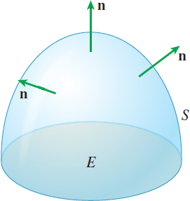
- Orientable. That is, it must be possible to choose a unit normal vector \mathbf{n} at each point of S, which we take as the positive direction of \mathbf{n}. The positively oriented vector \mathbf{n } must vary continuously, and as it moves around any closed curve on the surface, \mathbf{n} must return to its original direction.
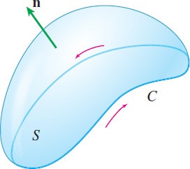
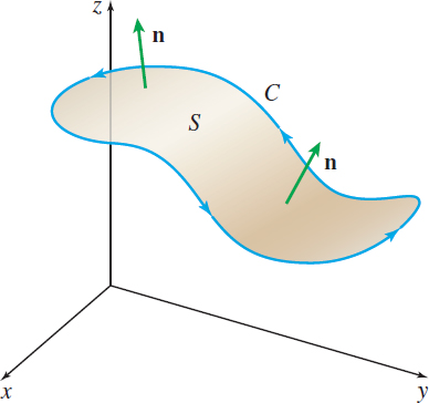
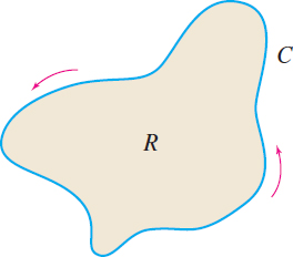
- The curve C of the line integral in (1) is a piecewise-smooth, simple closed curve that forms the boundary of the surface S. The positively oriented surface S induces a positive orientation on C in the sense that if you walk around C in the positive direction with your head pointing in the same direction as the unit normal \mathbf{n} to S, then the surface will always be to your left, as shown in Figure 71.
1047
THEOREM Stokes' Theorem
Let S be a smooth, simply connected, orientable surface bounded by a piecewise-smooth, simple closed curve C. Let \mathbf{F}=\mathbf{F} (x,y,z)=P(x,y,z)\mathbf{i}+Q(x,y,z)\mathbf{j}+R(x,y,z)\mathbf{k} be a vector field, where P, Q, and R have continuous first-order partial derivatives throughout a solid E containing S and C. Let \mathbf{n} denote the positive unit normal to S, and let C be positively oriented, as described earlier. Then {\bbox[#FAF8ED,5pt]{\bbox[5px, border:1px solid black, #F9F7ED]{ \oint_{C}\mathbf{F}\,{\bf\cdot}\, d\mathbf{r}=\iint\limits_{\kern-3ptS} {\rm{curl}\, \mathbf{F}\,{\bf\cdot}\, \mathbf{n}}\,dS}}}
In terms of the components of each vector, Stokes' Theorem takes the form {\bbox[5px, border:1px solid black, #F9F7ED]{\bbox[#FAF8ED,5pt]{ \oint\limits_{C}(P\,dx+Q\,dy+R\,dz)=\iint\limits_{\kern-3ptS}\left[ \left( \dfrac{ \partial R}{\partial y}-\dfrac{\partial Q}{\partial z}\right) dy\,dz-\left( \dfrac{\partial R}{\partial x}-\dfrac{\partial P}{\partial z} \right) \,dz\,dx+\left( \dfrac{\partial Q}{\partial x}-\dfrac{\partial P}{ \partial y}\right) dx\,dy\right]}}}
The proof of Stokes' Theorem is given in advanced calculus books.
2 Verify Stokes' TheoremPrinted Page 1047
EXAMPLE 2Verifying Stokes' Theorem
Verify Stokes' Theorem for \mathbf{F}=y\mathbf{i}-x\mathbf{j}, where the surface S is the paraboloid z=x^{2}+y^{2}, with x^{2}+y^{2}=1, z=1 , as its boundary C.
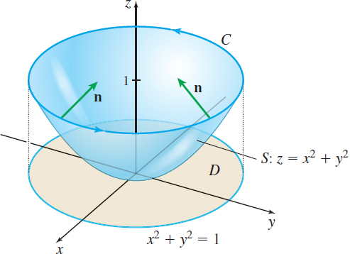
Solution Figure 72 shows the paraboloid and the circle C in the plane z=1. Stokes' Theorem states the following: \oint\limits_{C}\mathbf{F}\,{\bf\cdot}\, d\mathbf{r}=\iint\limits_{\kern-3ptS}{\rm{curl}\, \mathbf{F} \,{\bf\cdot}\, \mathbf{n}}\,dS
Parametric equations for C are x=\cos t, y=\sin t, z=1, 0\leq t\leq 2\pi. We use the parametric equations to find the line integral \oint_{C}\mathbf{F}\,{\bf\cdot}\, d\mathbf{r} for \mathbf{F}=y\mathbf{i}-x \mathbf{j}. \begin{eqnarray*} \oint_{C}\mathbf{F}\,{\bf\cdot}\, d\mathbf{r}&=&\oint_{C}(y\,dx-x\,dy)=\int_{0}^{2\pi } \left[ \sin t\left( -\sin t\,dt\right) -\cos t\cos t\,dt\right]\\[4pt] &=&-\int_{0}^{2\pi }[\sin ^{2}t+\cos ^{2}t]\,dt=-\int_{0}^{2\pi }dt=-2\pi \end{eqnarray*}
To find the surface integral, \iint\limits_{\kern-3ptS}{\rm{curl}\, \mathbf{F}\,{\bf\cdot}\, \mathbf{n}}\,dS, we find \rm{curl}\, \mathbf{F} and \mathbf{n}: \begin{eqnarray*} \rm{curl}\, \mathbf{F} &\mathbf{=}&\left\vert \begin{array}{@{}c@{\quad}c@{\quad}c} \mathbf{i} & \mathbf{j} & \mathbf{k} \\[3pt] \dfrac{\partial }{\partial x} & \dfrac{\partial }{\partial y} & \dfrac{\partial }{\partial z} \\[5pt] P & Q & R \end{array} \right\vert =\left\vert \begin{array}{@{}c@{\quad}c@{\quad}c} \mathbf{i} & \mathbf{j} & \mathbf{k} \\[3pt] \dfrac{\partial }{\partial x} & \dfrac{\partial }{\partial y} & \dfrac{\partial }{\partial z} \\[5pt] y & -x & 0 \end{array} \right\vert \\[4pt] &=&\left[ \dfrac{\partial }{\partial y}0-\dfrac{\partial }{\partial z}(-x) \right] \,\mathbf{i}-\left[ \dfrac{\partial }{\partial x}0-\dfrac{\partial }{ \partial z}y\right] \,\mathbf{j}+\left[ \dfrac{\partial }{\partial x}(-x)- \dfrac{\partial }{\partial y}y\right] \mathbf{k}\\[4pt] &=&0\mathbf{i}-0\mathbf{j}-2\mathbf{k}=-2\mathbf{k} \end{eqnarray*}
1048
For z=f(x,y) =x^{2}+y^{2}, we have \begin{eqnarray*} \mathbf{n\,} &=& \tfrac{-f_{x}(x,y)\mathbf{i}-f_{y}(x,y) \mathbf{j\,}+\,\mathbf{k}}{\sqrt{[f_{x}(x,y)]^{2}+[f_{y}(x,y)]^{2}+1}} = \dfrac{-2x\mathbf{i}-2y\mathbf{j}+\mathbf{k}}{\sqrt{ 4x^{2}+4y^{2}+1}}\\[4pt] \rm{curl}\, \mathbf{F}\,{\bf\cdot}\, \mathbf{n} &=&-2\mathbf{k\,{\bf\cdot}\, }\dfrac{1}{\sqrt{ 4x^{2}+4y^{2}+1}}\left( -2x\mathbf{i}-2y\mathbf{j}+\mathbf{k}\right) =\dfrac{ -2}{\sqrt{4x^{2}+4y^{2}+1}} \end{eqnarray*} So,
where D is the interior of the circle x^{2}+y^{2}=1.
NOW WORK
3 Use Stokes' Theorem to Find an IntegralPrinted Page 1048
EXAMPLE 3Using Stokes' Theorem to Find a Surface Integral
Find the surface integral \iint\limits_{\kern-3ptS}{\rm{curl} \, \mathbf{F}\,{\bf\cdot}\, \mathbf{n}}\,dS, where \mathbf{F}=\mathbf{F}(x,y,z)=y \mathbf{i}+x\mathbf{j}+z\mathbf{k} and S is the surface z=5-(x^{2}+y^{2}), z\geq 1, using Stokes' Theorem.
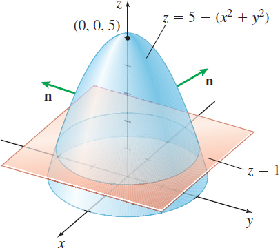
Solution Figure 73 shows the surface S. The boundary curve C is the circle x^{2}+y^{2}=4 that lies in the plane z=1. The vector form of C is \mathbf{r}=\mathbf{r}(t)=2\cos t\,\mathbf{i}+2\sin t\,\mathbf{j}+ \mathbf{k}, 0\leq t\leq 2\pi . Then \begin{eqnarray*} d\mathbf{r}& =&(-2\,\sin t\,\mathbf{i}+2\,\cos t\,\mathbf{j})\,dt \\[4pt] \mathbf{F}& =&y\mathbf{i}+x\mathbf{j}+z\mathbf{k}=2\,\sin t\mathbf{i}+2\,\cos t \mathbf{j}+\mathbf{k} \\[4pt] \mathbf{F}\,{\bf\cdot}\, d\mathbf{r}& =&(-4\,\sin ^{2}t+4\,\cos ^{2}t)\,dt=4\,\cos (2t) \,dt \end{eqnarray*}
Now we use Stokes' Theorem. \iint\limits_{\kern-3ptS}{\rm{curl}\, \mathbf{F}\,{\bf\cdot}\, \mathbf{n}}\,dS=\oint_{C}\mathbf{F} \,{\bf\cdot}\, d\mathbf{r}=\int_{0}^{2\pi }4\,\cos (2t) \,dt= 2 \big[ \sin(2t)\big] _{0}^{2\pi }=0
NOW WORK
In Example 3, we found the surface integral \iint\limits_{\kern-3ptS}\rm{curl}\, \mathbf{F}\,{\bf\cdot}\, \mathbf{n}\,dS using the line integral of \mathbf{F} on the boundary C of the surface S. This means that for any surface S_{1} with the same orientation and the same boundary curve as S, the surface integral \iint\limits_{\kern-3ptS_{1}}{\rm{curl}\, \mathbf{F}\,{\bf\cdot}\, \mathbf{n}}\,dS_{1} will have the same value as \iint\limits_{\kern-3ptS}{\rm{curl}\, \mathbf{F}\,{\bf\cdot}\, \mathbf{n}}\,dS.
We can use Stokes' Theorem to find a line integral, and avoid having to find a surface integral. However, it is more frequently used in the opposite direction. In cases where it is not easy to find the line integral \oint_{C}\mathbf{F}\,{\bf\cdot}\, d\mathbf{r}, but the quantity curl \mathbf{F} \,{\bf\cdot}\, \mathbf{n} is simple in form on an open surface with boundary C, then it can be easier to find \iint\limits_{\kern-3ptS}{\rm{curl}\, \mathbf{F}\,{\bf\cdot}\, \mathbf{n}}\,dS.
1049
EXAMPLE 4Using Stokes' Theorem to Find a Line Integral
Find I=\oint_{C}[(e^{-x^{2}/2}-yz)\,dx+(e^{-y^{2}/2}+xz+2x) \,dy+(e^{-z^{2}/2}+5)\,dz], where C is the circle x=\cos t, y=\sin t, z=2, 0\leq t\leq 2\pi .
Solution Let \mathbf{F}=P\,\mathbf{i}+Q\,\mathbf{j}+R\,\mathbf{k} , with P=e^{-x^{2}/2}-yz, \ Q=e^{-y^{2}/2}+xz+2x, and R=e^{-z^{2}/2}+5. It can be verified that {\rm{curl }}\,{\bf{F}} = - x{\bf{i}} - y{\bf{j}}{\rm{ + (2 + 2}}z){\bf{k}}
To use Stokes' Theorem, take S to be a plane region enclosed by the circle C in the plane z\rm{=2} so that \mathbf{n}=\mathbf{k}. Then \rm{curl}\, \mathbf{F}\,{\bf\cdot}\, \mathbf{n}=6 on S, and I=\iint\limits_{\kern-3pt S}{\rm{curl}\, \mathbf{F}\,{\bf\cdot}\, \mathbf{n}}\,dS=6\iint \limits_{\kern-3pt S}\,dx\,dy=6\,\pi
NOW WORK
4 Apply Stokes' Theorem to Conservative Vector FieldsPrinted Page 1049
A vector field \mathbf{F}=\mathbf{F}(x,y,z)=P(x,y,z)\mathbf{i}+Q(x,y,z) \mathbf{j}+R(x,y,z)\mathbf{k} is conservative if \mathbf{F} is the gradient of some function \omega =f(x,y,z). An extension of earlier proofs shows that \mathbf{F} is a conservative vector field if and only if \int_{C} \mathbf{F}\,{\bf\cdot}\, d\mathbf{r} is independent of the path, where C is a piecewise-smooth curve in space and \mathbf{F}=\mathbf{F}(x,y,z) is defined on some open, connected solid in space. In particular, if C is simple and closed, then \mathbf{F} is a conservative vector field if and only if \oint_{C}\mathbf{F}\,{\bf\cdot}\, d\mathbf{r}=0 for every piecewise-smooth, simple closed curve C.
Stokes' Theorem provides an easy way to determine whether a vector field \mathbf{F} in space is a conservative vector field.
THEOREM Conservative Vector Fields in Space
Let \mathbf{F}=P(x,y,z)\,\mathbf{i}+Q(x,y,z)\,\mathbf{j}+R(x,y,z)\, \mathbf{k} be a vector field whose components P, Q, and R have continuous first-order partial derivatives throughout a solid E whose boundary is a surface S satisfying the conditions of Stokes' Theorem. Then \mathbf{F} is a conservative vector field if and only if \rm{curl}\, \mathbf{F}=\mathbf{0} throughout S.
Partial Proof
We provide only an outline of the proof. Suppose \rm{curl}\, \mathbf{F}= \mathbf{0}. Then, by Stokes' Theorem, \begin{equation*} \oint_{C}\mathbf{F}\,{\bf\cdot}\, d\mathbf{r}=\iint\limits_{\kern-3ptS}{\rm{curl}\, \mathbf{F} \,{\bf\cdot}\, \mathbf{n}}\,dS=0 \end{equation*}
for any closed curve C. That is, \mathbf{F} is a conservative vector field.
Conversely, suppose \mathbf{F} is conservative. Then {\mathbf{F} = \bf\nabla} f for some function f. Since \mathbf{F}= \mathbf{F}(x,y,z)= P(x,y,z)\mathbf{i} + Q(x,y,z)\,\mathbf{j}+R(x,y,z)\,\mathbf{k}, and {\bf\nabla}f(x,y,z) = \dfrac{\partial }{\partial x} f(x,y,z)\mathbf{i} + \dfrac{\partial }{\partial y} f(x,y,z)\mathbf{j} + \dfrac{\partial }{\partial z}(x,y,z)\mathbf{k}, then \begin{eqnarray*} \rm{curl}\, \mathbf{F} &\mathbf{=}&\left\vert \begin{array}{@{}c@{\quad}c@{\quad}c} \mathbf{i} & \mathbf{j} & \mathbf{k} \\[3pt] \dfrac{\partial }{\partial x} & \dfrac{\partial }{\partial y} & \dfrac{\partial }{\partial z} \\[7pt] P & Q & R \end{array} \right\vert =\left\vert \begin{array}{@{}c@{\quad}c@{\quad}c} \mathbf{i} & \mathbf{j} & \mathbf{k} \\[3pt] \dfrac{\partial }{\partial x} & \dfrac{\partial }{\partial y} & \dfrac{\partial }{\partial z} \\[5pt] \dfrac{\partial }{\partial x}f(x,y,z) & \dfrac{\partial }{\partial y}f(x,y,z) & \dfrac{\partial }{\partial z}f(x,y,z) \end{array} \right\vert \\[6pt] &=& \left(\dfrac{\partial^{2}f }{\partial{y} \partial{z}} - \dfrac{\partial^{2}f }{\partial{z} \partial{y}}\right)\,\mathbf{i} - \left(\dfrac{\partial^{2}f }{\partial{x} \partial{z}} - \dfrac{\partial^{2}f }{\partial{z} \partial{x}}\right)\,\mathbf{j} + \left(\dfrac{\partial^{2}f }{\partial{x} \partial{y}} - \dfrac{\partial^{2}f }{\partial{y} \partial{x}}\right)\mathbf{k}\\[6pt] &=&0\mathbf{i}+0\mathbf{j}+0\mathbf{k}= \mathbf{0} \end{eqnarray*}
NEED TO REVIEW?
The Equality of Mixed Partials Theorem is discussed in Section 12.3, p. 835.
The following statements are similar to those listed in the Summary at the end of Section 15.3 for a vector field in the plane.
1050
Summary
Suppose \mathbf{F}=P(x,y,z)\,\mathbf{i}+Q(x,y,z)\,\mathbf{j}+R(x,y,z)\, \mathbf{k} is a vector field whose components P, Q, and R have continuous first-order partial derivatives throughout a solid E whose boundary is a smooth, simply connected, oriented surface S bounded by a piecewise-smooth, simple closed curve C. Then the following are equivalent statements for a vector field \mathbf{F}=P\mathbf{i}+Q\mathbf{j}+R\mathbf{k} in space:
- \mathbf{F} is a conservative vector field.
- \mathbf{F} is the gradient of some function.
- The work done by \mathbf{F} in moving an object of mass m from a point A to a point B in S is independent of the path from A to B.
- The work done by \mathbf{F} in moving an object of mass m along any piecewise-smooth, closed curve C in S is 0.
- \rm{curl}\,\mathbf{F=0}
Of all these equivalent statements, the easiest to establish is \rm{curl}\, \mathbf{F=0}.
EXAMPLE 5Showing That \mathbf{F} Is a Conservative Vector Field
Show that \mathbf{F}=\left( \dfrac{3}{5}y^{5}+2z^{2}\right) \mathbf{i} +3xy^{4}\,\mathbf{j}+4xz\,\mathbf{k} is a conservative vector field in space.
Solution We find \rm{curl}\, \mathbf{F}. \begin{equation*} \rm{curl}\, \mathbf{F}=\left\vert \begin{array}{@{}c@{\quad}c@{\quad}c} \mathbf{i} & \mathbf{j} & \mathbf{k} \\[5pt] \dfrac{\partial }{\partial x} & \dfrac{\partial }{\partial y} & \dfrac{ \partial }{\partial z} \\[5pt] \dfrac{3}{5}y^{5}+2z^{2} & 3xy^{4} & 4xz \end{array} \right\vert =(0-0)\,\mathbf{i}-(4z-4z)\,\mathbf{j}+(3y^{4}-3y^{4})\mathbf{k}= \mathbf{0} \end{equation*}
Since \rm{curl}\,\mathbf{F=0}, \mathbf{F} is conservative.
NOW WORK
5 Interpret the Curl of F
Printed Page 1050
Stokes' Theorem provides an interpretation for the curl of a vector.
Suppose Q=(x_{1},y_{1},z_{1}) is the center of a circular disk S_{\rho } of radius \rho and C_{\rho } is the boundary of S_{\rho }, as shown in Figure 74. There is a Mean Value Theorem for double integrals that, when combined with Stokes' Theorem, gives us {\bbox[5px, border:1px solid black, #F9F7ED]{\bbox[#FAF8ED,5pt]{ \oint\limits_{C_{\rho }}\mathbf{F}\,{\bf\cdot}\, d\mathbf{r}=\iint\limits_{\kern-3ptS_{ \rho }}{\rm{curl}\, \mathbf{F}\,{\bf\cdot}\, \mathbf{n}}\,dS=\left(\rm{curl}\,\mathbf{ F\,{\bf\cdot}\, n}\right) _{Q^{\ast }}( \pi \rho ^{2})}}}
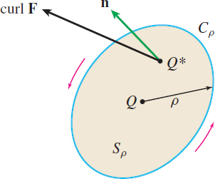
where \left( \rm{curl}\, \mathbf{F}\,{\bf\cdot}\, \mathbf{n}\right) _{Q^{\ast }} is the value of \rm{curl}\, \mathbf{F}\,{\bf\cdot}\, \mathbf{n} evaluated at a suitably chosen point Q^{\ast }=(x^{\ast },y^{\ast },z^{\ast }) in S_{\rho }, and where \pi \rho ^{2} is the area of S_{\rho }. Then \begin{equation*} (\rm{curl}\, \mathbf{F}\,{\bf\cdot}\, \mathbf{n})_{Q^{\ast }}=\dfrac{1}{\pi \rho ^{2}} \oint_{C_{\rho }}\mathbf{F}\,{\bf\cdot}\, d\mathbf{r} \end{equation*}
Now, if \rho is allowed to approach 0, then Q^{\ast }\rightarrow Q, and \begin{equation} (\rm{curl}\, \mathbf{F}\,{\bf\cdot}\, \mathbf{n})_{Q}=\lim\limits_{\rho \rightarrow 0}\dfrac{1 }{\pi \rho ^{2}}\oint_{C_{\rho }}\mathbf{F}\,{\bf\cdot}\, d\mathbf{r} \tag{2} \end{equation}
In the case where \mathbf{F} is the velocity of a fluid, the integral \oint_{C_{\rho }}\mathbf{F}\,{\bf\cdot}\, d\mathbf{r} in (2) is referred to as the circulation, or whirling tendency of the fluid around C_{\rho}. It measures the extent to which the fluid rotates around the circle C_{\rho } in the direction of the orientation of C_{\rho }. Equation (2) therefore states that the component of \rm{curl}\, \mathbf{F} at (x_{1},y_{1},z_{1}) in the direction of \mathbf{n} is the limiting ratio of circulation to area for a circle about (x_{1},y_{1},z_{1}) with \mathbf{n} as a normal, or {\bbox[5px, border:1px solid black, #F9F7ED]{\bbox[#FAF8ED,5pt]{ \hbox{Circulation per unit of area at } ( x_{1},y_{1},z_{1}) =(\rm{curl}\, \mathbf{F}\,{\bf\cdot}\, \mathbf{n})_{Q} }}}
The expression (\rm{curl}\, \mathbf{F}\,{\bf\cdot}\, \mathbf{n})_{Q} is a maximum at Q when \mathbf{n} has the same direction as curl \mathbf{F}.
1051
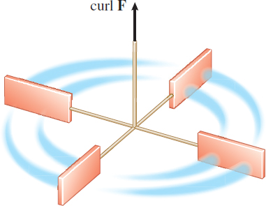


Suppose that a small paddle wheel of radius \rho is introduced into the fluid at Q with its axle directed along \mathbf{n}. The rate of spin of the paddle wheel is affected by the circulation of the fluid around C_{\rho }. The wheel will spin fastest when the circulation integral is maximized; that is, it will spin fastest when the axle of the paddle wheel is in the direction of \rm{curl}\,\mathbf{F}. See Figure 75.
Another interpretation of the curl is based on motion.
THEOREM Curl and Angular Velocity
Let \mathbf{F} be the velocity field of a fluid rotating about a fixed axis and let {\bf\omega } be the constant angular velocity. Then {\bbox[5px, border:1px solid black, #F9F7ED]{\bbox[#FAF8ED,5pt]{ \rm{curl}\, \mathbf{F}=2 \bf\omega }}}
NEED TO REVIEW?
Angular velocity is discussed in Section 10.5, pp. 729-730.
Proof
Since the motion of a fluid is simply a rotation about a given fixed axis in space, the angular velocity {\bf\omega } can be represented by a constant vector: {\bf\omega }=\omega _{1}\mathbf{i}+\omega _{2}\mathbf{j}+\omega _{3}\mathbf{k}
where the magnitude of {\bf\omega } is the angular speed and the direction of {\bf\omega } is along the direction of the axis of rotation, in accordance with the right-hand rule. If the origin of a rectangular coordinate system is on the fixed axis and \mathbf{r}=x\mathbf{i }+y\mathbf{j}+z\mathbf{k}, then the velocity vector \mathbf{F} is \mathbf{F}={\bf\omega} \times \mathbf{r} and \rm{curl}\, \mathbf{F}=\left\vert \begin{array}{@{}c@{\quad}c@{\quad}c} \mathbf{i} & \mathbf{j} & \mathbf{k} \\[3pt] \dfrac{\partial }{\partial x} & \dfrac{\partial }{\partial y} & \dfrac{\partial }{\partial z} \\[3pt] \omega _{2}z-\omega _{3}y & \omega _{3}x-\omega _{1}z & \omega _{1}y-\omega _{2}x \end{array} \right\vert
Since {\bf\omega } is constant, then \rm{curl}\, \mathbf{F}=2\omega _{1}\mathbf{i}+2\omega _{2}\mathbf{j}+2\omega _{3}\mathbf{k}=2 {\bf\omega }
IN WORDS
If a fluid is rotating, the curl of the velocity vector is a constant vector that equals twice the angular velocity vector.
Summary
We opened the chapter by stating that “vector calculus is the culmination of what we have learned throughout the course.” Now we end the chapter with a list of several of the formulas we have learned. The theorem formulas given below do not contain the important hypotheses necessary for the formulas to hold. Rather, this summary is meant to “pull everything together” and provide “the big picture of calculus.”
Fundamental Theorem of Line Integrals
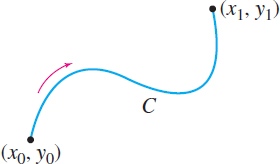
If {{\bf}{\nabla}} \,f(x,\,y) = {\bf{F}}(x,\,y), then \int_{C}\mathbf{F}\,{\bf\cdot}\, d\mathbf{r}=\int_{C} {\bf\nabla}\ f\,{\bf\cdot}\, d\mathbf{r}=\int_{(x_{0},y_{0}) }^{(x_{1},y_{1}) }{\bf\nabla}\ f\,{\bf\cdot}\, d\mathbf{r}=f(x_{1},y_{1}) -f(x_{0},y_{0})
Fundamental Theorem of Calculus
If F' (x) =f(x) , then \int_{a}^{b}f(x) dx=\int_{a}^{b}F' (x) dx=F( b) -F( a)
Green's Theorem
If \mathbf{F}(x,y) =P(x,y) \,\mathbf{i}+Q(x,y) \,\mathbf{j}, then \oint_{C}\mathbf{F}\,{\bf\cdot}\, d\mathbf{r} =\oint_{C}(P\,dx+Q\,dy)=\iint\limits_{\kern-3ptR}\left( \dfrac{\partial Q}{\partial x} -\dfrac{\partial P}{\partial y}\right) \,dx\,dy
1052
Divergence Theorem
If \mathbf{F}(x,y,z)=P(x,y,z)\mathbf{i}+Q(x,y,z)\mathbf{j}+R(x,y,z)\mathbf{k}, and \mathbf{n}=\cos \alpha \mathbf{i}+\cos \beta \mathbf{j}+\cos \gamma \mathbf{k}, then \begin{eqnarray*} &&\iiint\limits_{E}{\rm div}\,\mathbf{F}\,dV = \iint\limits_{\kern-3ptS}\mathbf{F}\,{\bf\cdot}\, {\mathbf{n}}\,dS \\ &&\iiint\limits_{E}\left( \dfrac{\partial P}{\partial x}+ \dfrac{\partial Q}{\partial y}+\dfrac{\partial R}{\partial z} \right) dV\\[4pt] &&\hspace{7pc}=\iint\limits_{S}(P\cos \alpha +Q\cos \beta +R\cos \gamma )\,dS \end{eqnarray*}
Stokes' Theorem
If \mathbf{F}(x,y,z)=P(x,y,z)\mathbf{i}+Q(x,y,z)\mathbf{j}+R(x,y,z)\mathbf{k}, then \begin{eqnarray*} &&\oint_{C}\mathbf{F}\,{\bf\cdot}\, d\mathbf{r}=\iint\limits_{S}{\rm{curl}\, \mathbf{F}\,{\bf\cdot}\, \mathbf{n}}\,dS \\ &&\hspace{.5pc}\oint_{C}(P\,dx+Q\,dy+R\,dz)=\iint\limits_{S}\left[ \left( \dfrac{\partial R}{\partial y}-\dfrac{\partial Q}{\partial z}\right) dy\,dz\right.\hspace{-2.6pc}\\ &&\qquad-\left.\left( \dfrac{\partial R}{\partial x}-\dfrac{\partial P}{\partial z} \right) dz\,dx+\left( \dfrac{\partial Q}{\partial x}-\dfrac{\partial P}{ \partial y}\right) dx\,dy\right] \end{eqnarray*}