1.4 Limits and Continuity of Trigonometric, Exponential, and Logarithmic FunctionsPrinted Page 106
OBJECTIVES
When you finish this section, you should be able to:
We have found limits using the basic limits lim and \lim\limits_{x\rightarrow c}x=c and properties of limits. But there are many limit problems that cannot be found by directly applying these techniques. To find such limits requires different results, such as the Squeeze Theorem *, or basic limits involving trigonometric and exponential functions.
*The Squeeze Theorem is also known as the Sandwich Theorem and the Pinching Theorem.
1 Use the Squeeze Theorem to Find a LimitPrinted Page 106
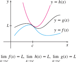
To use the Squeeze Theorem to find \lim\limits_{x\rightarrow c}g(x), we need to know, or be able to find, two functions f and h that “sandwich” the function g between them for all x close to c. That is, in some interval containing c, the functions f, g, and h satisfy the inequality f( x) \leq g( x) \leq h( x). Then if f and h have the same limit L as x approaches c, the function g is “squeezed” to the same limit L as x approaches c. See Figure 37.
We state the Squeeze Theorem here. The proof is given in Appendix B.
107
THEOREM Squeeze Theorem
Suppose the functions f, g, and h have the property that for all x in an open interval containing c, except possibly at c, \begin{equation*} f(x)\leq g(x)\leq h(x)\ \end{equation*}
If \begin{equation*} \lim_{x\rightarrow c}f(x)=\lim_{x\rightarrow c}h(x)=L\ \end{equation*}
then \begin{equation*} \lim_{x\rightarrow c}g(x)=L\ \end{equation*}
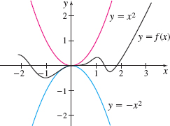
For example, suppose we wish to find \lim\limits_{x\rightarrow 0}f(x), and we know that -x^{2}\leq f(x)\leq x^{2} for all x\neq 0. Since \lim\limits_{x\rightarrow 0}({-x^{2}}) =0 and \lim\limits_{x\rightarrow 0}x^{2}=0, the Squeeze Theorem tells us that \lim\limits_{x\rightarrow 0}f(x)=0. Figure 38 illustrates how f is “squeezed” between y=x^{2} and y=-x^{2} near 0.
EXAMPLE 1Using the Squeeze Theorem to Find a Limit
Use the Squeeze Theorem to find \lim\limits_{x\rightarrow 0}\left( x\sin \dfrac{1}{x}\right).
Solution If x\neq 0, then \sin \dfrac{1}{x} is defined. We seek two functions that “squeeze” y=x\sin \dfrac{1}{x} near 0. Since -1\leq \sin x\leq 1 for all x, we begin with the inequality \begin{equation*} \left\vert \sin \dfrac{1}{x}\right\vert \leq 1\qquad x\neq 0 \end{equation*}
Since x\neq 0 and we seek to squeeze x\sin \dfrac{1}{x}, we multiply both sides of the inequality by \vert x\vert , x\neq 0. Since \vert x\vert >0, the direction of the inequality is preserved. Note that if we multiply \left\vert \sin \dfrac{1}{x}\right\vert \leq 1 by x, we would not know whether the inequality symbol would remain the same or be reversed since we do not know whether x>0 or x\lt 0. \begin{equation*} \begin{array}{r@{\qquad}ll} |x|\left\vert \sin \dfrac{1}{x}\right\vert \leq |x| & & {\color{#0066A7}{\hbox{Multiply both sides by \(\vert x \vert >0\).}}} \\[12pt] \left\vert x\sin \dfrac{1}{x}\right\vert \leq |x| & & {\color{#0066A7}{{|a|\cdot |b| = |a\,b|}.}} \\[11pt] -\vert x\vert \leq x\sin \dfrac{1}{x}\leq |x| & & {\color{#0066A7}{\vert a\vert\,{\leq}\,b\hbox{ is equivalent to } {-b\leq a\leq b.}}} \end{array} \end{equation*}
Now use the Squeeze Theorem with f(x) = - |x|, g(x) = x\sin \dfrac{1}{x}, and h(x) = |x|. Since f(x)\leq g(x)\leq h(x) and \begin{equation*} \lim_{x\rightarrow 0}f(x)=\lim_{x\rightarrow 0}(-|x|)=0\qquad \hbox{and}\qquad \lim_{x\rightarrow 0}h(x)=\lim_{x\rightarrow 0}\vert x\vert =0 \end{equation*}
it follows that \lim_{x\rightarrow 0}g(x)=\lim_{x\rightarrow 0}\left( x\cdot \sin \frac{1}{x} \right) =0
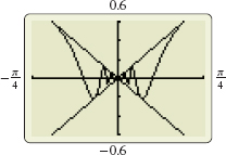
Figure 39 illustrates how g( x) =x\sin \dfrac{1}{x} is squeezed between y=-\vert x\vert and y=\vert x\vert.
NOW WORK
2 Find Limits Involving Trigonometric FunctionsPrinted Page 108
108
Knowing \lim\limits_{x\rightarrow c}A = A and \lim\limits_{x\rightarrow c}x = c helped us to find the limits of many algebraic functions. Knowing several basic trigonometric limits can help to find many limits involving trigonometric functions.
THEOREM Two Basic Trigonometric Limits
\bbox[5px, border:1px solid black, #F9F7ED]{\lim\limits_{x \rightarrow 0}\sin x=0 \qquad \lim\limits_{x\rightarrow 0}\cos x=1}
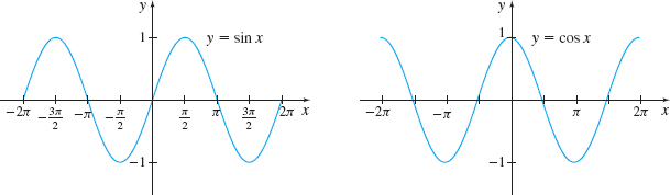
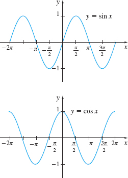
The graphs of y = \sin x and y = \cos x in Figure 40 illustrate that \lim\limits_{x\rightarrow 0}\sin x = 0 and \lim\limits_{x\rightarrow 0}\cos x = 1. The proofs of these limits both use the Squeeze Theorem. Problem 64 provides an outline of the proof that \lim\limits_{x\rightarrow 0}\sin x = 0.
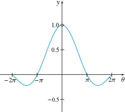
A third basic trigonometric limit, \lim\limits_{\theta \rightarrow 0}\dfrac{\sin \theta}{\theta} = 1, is important in calculus. In Section 1.1, a table of numbers suggested that \lim\limits_{\theta \rightarrow 0}\dfrac{\sin\theta}{\theta} = 1. The function f(\theta) = \dfrac{\sin\theta}{\theta}, whose graph is given in Figure 41, is defined for all real numbers \theta \neq 0. The graph suggests \lim\limits_{\theta\rightarrow 0}\dfrac{\sin \theta}{\theta} = 1.
THEOREM
If \theta is measured in radians, then \bbox[5px, border:1px solid black, #F9F7ED]{ \lim\limits_{\theta \rightarrow 0}\dfrac{\sin \theta }{\theta }=1}
Proof
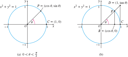
Although \dfrac{\sin \theta}{\theta} is a quotient, we have no way to divide out \theta. To find \lim\limits_{\theta \rightarrow 0^{+}}\dfrac{\sin \theta}{\theta}, we let \theta be a positive acute central angle of a unit circle, as shown in Figure 42(a). Notice that {\it COP} is a sector of the circle. We add the point B = (\cos \theta ,0) to the graph and form triangle BOP. Next we extend the terminal side of angle \theta until it intersects the line x = 1 at the point D, forming a second triangle COD. The x-coordinate of D is 1. Since the length of the line segment \overline{OC} is {OC} = 1, then the y-coordinate of D is {CD} = \dfrac{{CD}}{{OC}} = \tan \theta. So, D = (1,\tan \theta). See Figure 42(b).
109
We see from Figure 42(b) that
area of triangle BOP≤ area of sector COP≤ area of triangle COD \tag{1}
Each of these areas can be expressed in terms of \theta as \begin{array}{l@{\quad}l} \hbox{area of triangle}{\it BOP} = \dfrac{1}{2}\cos \theta \cdot \sin \theta & {\color{#0066A7}{\hbox{area of a triangle $ = \dfrac{1}{2}$ base $\times$ height}}}\\[6pt] \hbox{area of sector}{\it COP} = \dfrac{\theta}{2} & {\color{#0066A7}{\hbox{area of sector $A = \dfrac{1}{2}{r}^{2}{\theta}$; $r = 1$}}}\\[6pt] \hbox{area of triangle}{\it COD} = \dfrac{1}{2}\cdot 1\cdot \tan \theta = \dfrac{ \tan \theta}{2} & {\color{#0066A7}{\hbox{area of a triangle $ = \dfrac{1}{2}$ base $\times$ height}}} \end{array}
So, for 0\lt \theta \lt \dfrac{\pi}{2}, we have \begin{equation*} \begin{array}{@{\;}rcl@{\quad}l} \!\!\dfrac{1}{2}\cos \theta \cdot \sin \theta &\leq& \dfrac{\theta}{2}\leq \dfrac{ \tan \theta}{2} & {\color{#0066A7}{\hbox{(1)}}} \\[10pt] &&&\quad \\ \cos \theta \cdot \sin \theta &\leq& \theta \leq \dfrac{\sin \,\theta}{\cos \theta} & {\color{#0066A7}{\hbox{Multiply all parts by 2; $\tan \theta = \dfrac{\sin \theta}{\cos \theta}$.}}}\\[11pt] \cos \theta &\leq& \dfrac{\theta}{\sin \theta}\leq \dfrac{1}{\cos \theta} & {\color{#0066A7}{\hbox{Divide all parts by $\sin \theta$; since $0 \lt \theta \lt \dfrac{\pi}{2}, \sin \theta >0$.}}} \\[10pt] \dfrac{1}{\cos \theta}&\geq& \dfrac{\sin \theta}{ \theta}\geq \cos \theta & {\color{#0066A7}{\hbox{Invert each term in the inequality; change the inequality signs.}}}\\[-2.5pt] \cos \theta &\leq& \dfrac{\sin \theta}{\theta} \leq \dfrac{1}{\cos \theta} & {\color{#0066A7}{\hbox{Rewrite using $\leq$.}}} \end{array} \end{equation*}
Now we use the Squeeze Theorem with f(\theta) = \cos \theta, \ g(\theta) = \dfrac{\sin \theta}{\theta}, and h(\theta) = \dfrac{1}{\cos \theta}. Since f(\theta)\leq \,g(\theta)\leq h(\theta), and since \begin{equation*} \lim_{\theta \rightarrow 0^{+}}f(\theta) = \lim_{\theta \rightarrow 0^{+}}\cos \theta = 1\quad \hbox{and}\quad \lim_{\theta \rightarrow 0^{+}}h(\theta) = \lim_{\theta \rightarrow 0^{+}}\frac{1}{\cos \theta} = \frac{\lim\limits_{\theta \rightarrow 0^{+}}1}{\lim\limits_{\theta \rightarrow 0^{+}}\cos \theta} = \frac{1}{1} = 1 \end{equation*} then by the Squeeze Theorem, \lim\limits_{\theta \rightarrow 0^{+}}g(\theta) = \lim\limits_{\theta \rightarrow 0^{+}}\dfrac{\sin \theta}{\theta} = 1.
Now we use the fact that g(\theta) = \dfrac{\sin \theta}{\theta} is an even function, that is, g(-\theta) = \dfrac{\sin \left(-\theta \right)}{-\theta} = \dfrac{ -\sin \theta}{-\theta} = \dfrac{\sin \theta}{\theta} = g(\theta)
So, \begin{equation*} \lim\limits_{\theta \rightarrow 0^{-}}\dfrac{\sin \theta}{\theta} = \lim\limits_{\theta \rightarrow 0^{+}}\dfrac{\sin \left(-\theta \right) }{-\theta} = \lim\limits_{\theta \rightarrow 0^{+}}\dfrac{\sin \theta}{ \theta} = 1 \end{equation*}
It follows that \lim\limits_{\theta \rightarrow 0}\dfrac{\sin \theta}{\theta} = 1.
110
Since \lim\limits_{\theta \rightarrow 0}\dfrac{\sin \theta}{\theta} = 1, the ratio \dfrac{\sin \theta}{\theta} is close to 1 for values of \theta close to 0. That is, \sin \theta \approx \theta for values of \theta close to 0. Table 9 illustrates this property.
| x near 0 on the left | x near 0 on the right | |||||||
|---|---|---|---|---|---|---|---|---|
| \theta (radians) | -0.5 | -0.1 | -0.01 | -0.001 | 0.001 | 0.01 | 0.1 | 0.5 |
| \sin \theta | -0.4794 | -0.0998 | -0.010 | -0.001 | 0.001 | 0.010 | 0.0998 | 0.4794 |
The basic limit \lim\limits_{\theta \rightarrow 0}\dfrac{\sin \theta}{ \theta} = 1 can be used to find the limits of similar expressions.
EXAMPLE 2Finding the Limit of a Trigonometric Function
Find:
- (a) \lim\limits_{\theta \rightarrow 0}\dfrac{\sin (3\theta)}{\theta}
- (b) \lim\limits_{\theta \rightarrow 0}\dfrac{\sin (5\theta)}{\sin (2\theta)}
Solution (a) Since \lim\limits_{\theta \rightarrow 0}\dfrac{\sin (3\theta)}{\theta} is not in the same form as \lim\limits_{\theta\rightarrow 0}\dfrac{\sin \theta}{\theta}, we multiply the numerator and the denominator by 3, and make the substitution t = 3\theta. \begin{equation*} \lim_{\theta \rightarrow 0}\frac{\sin (3\theta )}{\theta }=\lim_{\theta \rightarrow 0}\frac{3\sin (3\theta )}{3\theta } \underset{\color{#0066A7}{{t\rightarrow 0}{\hbox{ as }}{\theta \rightarrow 0}}}{\underset{\color{#0066A7}{{t=3\theta}}}{\underset{\color{#0066A7}{\uparrow }}{=}}} \lim_{t\rightarrow 0}\left( 3\frac{\sin t}{t}\right) =3\lim_{t\rightarrow 0} \frac{\sin t}{t}\underset{\color{#0066A7}{{\lim\limits_{t\rightarrow 0}\dfrac{\sin t}{t}=1 }}}{\underset{\color{#0066A7}{\uparrow }}{=}}\!\!(3)(1)=3 \end{equation*}
(b) We begin by dividing the numerator and the denominator by \theta. Then \begin{equation*} \dfrac{\sin (5\theta)}{\sin (2\theta)} = \dfrac{ \dfrac{\sin (5\theta)}{\theta}}{\dfrac{\sin (2\theta)}{\theta}} \end{equation*}
Now we follow the approach in (a) on the numerator and on the denominator. \begin{eqnarray*} \lim\limits_{\theta \rightarrow 0}\dfrac{\sin ( 5\theta ) }{ \theta } &=&\lim\limits_{\theta \rightarrow 0}\dfrac{5\sin ( 5\theta ) }{5\,\theta } \underset{\color{#0066A7}{{t\rightarrow 0\hbox{ as }\theta \rightarrow 0}}} {\underset{\color{#0066A7}{t=5\theta}}{\underset{\color{#0066A7}{\uparrow }}{=}}}\lim\limits_{t\rightarrow 0} \dfrac{5\sin t}{t}=5\lim\limits_{t\rightarrow 0}\left( \dfrac{\sin t}{t} \right) =5 \\ \lim\limits_{\theta \rightarrow 0}\dfrac{\sin ( 2\theta ) }{ \theta } &=&\lim\limits_{\theta \rightarrow 0}\dfrac{2\sin ( 2\theta ) }{2\theta } \underset{\color{#0066A7}{{t\rightarrow 0\hbox{ as }\theta \rightarrow 0}}}{ \underset{\color{#0066A7}{{t=2\theta}}}{\underset{\uparrow }{=}}}\lim\limits_{t\rightarrow 0}\left( \dfrac{2\sin t}{t}\right) =2\lim\limits_{t\rightarrow 0}\dfrac{\sin t}{t}=2 \\ \lim\limits_{\theta \rightarrow 0} \dfrac{\sin (5\theta)}{\sin (2\theta)} &=&\dfrac{ \lim\limits_{\theta \rightarrow 0}\dfrac{\sin (5\theta)}{\theta}}{\lim\limits_{\theta \rightarrow 0}\dfrac{\sin (2\theta)}{\theta}} = \frac {5}{2} \end{eqnarray*}
NOW WORK
Example 3 establishes an important limit used in Chapter 2.
111
EXAMPLE 3Finding a Basic Trigonometric Limit
Establish the formula \bbox[5px, border:1px solid black, #F9F7ED]{ \lim\limits_{\theta \rightarrow 0}\dfrac{\cos \theta -1}{\theta} = 0}
where \theta is measured in radians.
Solution First we rewrite the expression \dfrac{\cos \theta -1}{\theta} as the product of two terms whose limits are known. For \theta \neq 0, \begin{eqnarray*} \frac{\cos \theta -1}{\theta }&=&\left( \frac{\cos \theta -1}{\theta }\right)\! \left( \frac{\cos \theta +1}{\cos \theta +1}\right)\\ &=&\frac{\cos ^{2}\theta -1 }{\theta (\cos \theta +1)}\underset{\color{#0066A7}{{\sin ^{2}{\theta +}\cos ^{2} {\theta =1}}}}{\underset{\color{#0066A7}{\uparrow }}{=}}\frac{-\sin ^{2}\theta }{\theta (\cos \theta +1)} = \left( \frac{\sin \theta }{\theta }\right) \frac{(-\sin \theta)}{\cos \theta +1} \end{eqnarray*}
Now we find the limit. \begin{eqnarray*} \lim_{\theta \rightarrow 0}\frac{\cos \theta -1}{\theta } &=&\lim_{\theta \rightarrow 0}\left[ \left( \frac{\sin \theta }{\theta } \right) \!\left( \frac{(-\sin \theta )}{\cos \theta +1}\right) \right] = \left[ \lim_{\theta \rightarrow 0}\frac{ \sin \theta }{\theta }\right]~ \!\left[ \lim_{\theta \rightarrow 0} \frac{ -\sin\theta}{\cos \theta +1} \right] \nonumber \\ &=& 1\,{\cdot}\,\dfrac{\lim\limits_{\theta \rightarrow 0}(-\sin \theta)}{\lim\limits_{\theta \rightarrow 0}(\cos\theta+1)} =\dfrac{0}{2} =0 \end{eqnarray*}
NOW WORK
3 Determine Where the Trigonometric Functions Are ContinuousPrinted Page 111
The graphs of f(x) = \sin x and g(x) = \cos x shown on the left suggest that f and g are continuous on their domains, the set of all real numbers.
EXAMPLE 4Showing f(x) = sin x Is Continuous at 0
- f(0) = \sin 0 = 0, so f is defined at 0.
- \lim\limits_{x\rightarrow 0}f(x) = \lim\limits_{x\rightarrow 0}\sin x = 0, so the limit at 0 exists.
- \lim\limits_{x\rightarrow 0}\sin x = \sin 0 = 0.
Since all three conditions of continuity are satisfied, f(x) = \sin x is continuous at 0.
In a similar way, we can show that g(x) = \cos x is continuous at 0. That is, \lim\limits_{x\rightarrow 0}\cos x = \cos 0 = 1.
You are asked to prove the following theorem in Problem 68.
THEOREM
- The sine function y = \sin x is continuous on its domain, all real numbers.
- The cosine function y = \cos x is continuous on its domain, all real numbers.
Based on this theorem the following two limits can be added to the list of basic limits. \bbox[5px, border:1px solid black, #F9F7ED]{ \lim\limits_{x\rightarrow c}\sin x = \sin c\qquad \hbox{ for all real numbers} c} \bbox[5px, border:1px solid black, #F9F7ED]{ \lim\limits_{x\rightarrow c}\cos x = \cos c\qquad \hbox{ for all real numbers} c}
112
EXAMPLE 5Application: Projectile Motion
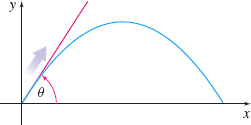


An object is propelled from ground level at an angle \theta , 0\lt \theta \lt \dfrac{\pi}{2}, to the horizontal with an initial velocity of 16feet/second, as shown in Figure 43. The equations of the horizontal position x = x(\theta) and the vertical position y = y(\theta) of the object after t seconds are given by \begin{equation*} x = x(\theta) = (16\cos \theta) t\qquad \hbox{and}\qquad y = y(\theta) = -16t^{2}+(16\sin \theta) t \end{equation*}
For a fixed time t:
- (a) Find \lim\limits_{\theta \rightarrow 0^{+}}x(\theta) and \lim\limits_{\theta \rightarrow 0^{+}}y(\theta).
- (b) Are the limits found in (a) consistent with what is expected physically?
- (c) Find \lim\limits_{\theta \rightarrow \frac{\pi}{2}^{-}}x(\theta) and \lim\limits_{\theta \rightarrow \frac{\pi}{2}^{-}}y(\theta).
- (d) Are the limits found in (c) consistent with what is expected physically?
Solution (a) \begin{eqnarray*} \lim\limits_{\theta \rightarrow 0^{+}}x(\theta) &=&\Big[\lim\limits_{\theta \rightarrow 0^{+}}(16\cos \theta)\Big] t = 16t\qquad{\color{#0066A7}{\hbox{$t$ fixed}}}\\[3pt] \lim\limits_{\theta \rightarrow 0^{+}}y(\theta) &=&\lim\limits_{\theta \rightarrow 0^{+}} [ -16t^{2}+(16\sin \theta) t ]\\[3pt] &=&\lim\limits_{\theta \rightarrow 0^{+}}(-16t^{2}) +\Big[\lim\limits_{\theta \rightarrow 0^{+}}(16\sin \theta)\Big] t = -16t^{2} \end{eqnarray*}
(b) The limits in (a) tell us that the horizontal position x of the object moves to the right (x = 16t) over time and that the vertical position y of the object immediately moves downward (y = -16t^{2}) into the ground. Neither of these conclusions is consistent with what we expect from the motion of an object propelled at an angle close to \theta = 0.
(c) \begin{eqnarray*} \lim\limits_{\theta \rightarrow \frac{\pi}{2}^{-}}x(\theta) &=&\Big[\lim\limits_{\theta \rightarrow \frac{\pi}{2}^{-}}(16\cos \theta)\Big] t = 0\\[3pt] \lim\limits_{\theta \rightarrow \frac{\pi}{2}^{-}}y(\theta) &=&\lim\limits_{\theta \rightarrow \frac{\pi}{2}^{-}}\left[ -16t^{2}+(16\sin \theta) t\right] = \lim\limits_{\theta \rightarrow \frac{\pi}{2}^{-}}(-16t^{2}) +\Big[\lim\limits_{\theta \rightarrow \frac{\pi}{2}^{-}}(16\sin \theta)\Big] t\\[3pt] &=&-16t^{2}+16t \end{eqnarray*}
(d) The limits we found in (c) tell us that the horizontal position remains at 0. The vertical position y = -16t^{2}+16t = -16t(t-1) tells us the object has a maximum height of 4feet and returns to the ground after 1 second. (The parabola y = -16t^{2}+16t opens down and has a maximum value at t = \dfrac{-b}{2a} = \dfrac{-16}{-32} = \dfrac{1}{2} at which time y = 4.) These conclusions are consistent with what we would expect from the motion of an object propelled close to the vertical.
NOW WORK
Using the facts that the sine and cosine functions are continuous for all real numbers, we can use basic trigonometric identities to determine where the remaining four trigonometric functions are continuous:
- y = \tan x: Since \tan x = \dfrac{\sin x}{\cos x}, from the Continuity of a Quotient property, y = \tan x is continuous at all real numbers except those for which \cos x = 0. That is, it is continuous on its domain, all real numbers except odd multiples of \dfrac{\pi}{2}.
- y = \sec x: Since \sec x = \dfrac{1}{\cos x}, from the Continuity of a Quotient property, y = \sec x is continuous at all real numbers except those for which \cos x = 0. That is, it is continuous on its domain, all real numbers except odd multiples of \dfrac{\pi}{2}.
y = \cot x: Since \cot x = \dfrac{\cos x}{\sin x}, from the Continuity of a Quotient property, y = \cot x is continuous at all real numbers except those for which \sin x = 0.
113
That is, it is continuous on its domain, all real numbers except integer multiples of \pi.
- y = \csc x: Since \csc x = \dfrac{1}{\sin x}, from the Continuity of a Quotient property, y = \csc x is continuous at all real numbers except those for which \sin x = 0. That is, it is continuous on its domain, all real numbers except integer multiples of \pi .
Recall that a one-to-one function that is continuous on its domain has an inverse function that is continuous on its domain.
NEED TO REVIEW?
Inverse trigonometric functions are discussed in Section P.7, pp. 58-63.
Since each of the six trigonometric functions is continuous on its domain, then each is continuous on the restricted domain used to define its inverse trigonometric function. This means the inverse trigonometric functions are continuous on their domains. These results are summarized in Table 10.
| Function | Domain | Properties |
|---|---|---|
| Sine | all real numbers | continuous on the interval (-\infty ,\infty) |
| Cosine | all real numbers | continuous on the interval (-\infty ,\infty) |
| Tangent | \left\{ x|x\neq\hbox{odd integer multiples of}\dfrac{\pi}{2}\right\} | continuous at all real numbers except odd multiples of \dfrac{\pi}{2}} |
| Cosecant | {x|x\neq integer multiples of π} | continuous at all real numbers except multiples of \pi |
| Secant | \left\{ x|x\neq \hbox{ odd integer multiples of}\dfrac{\pi}{2}\right\} | continuous at all real numbers except odd multiples of \dfrac{\pi}{2} |
| Cotangent | { x|x \neq integer multiples of π} | continuous at all real numbers except multiples of \pi |
| Inverse sine | -1\leq x\leq 1 | continuous on the closed interval [ -1,1] |
| Inverse cosine | -1\leq x\leq 1 | continuous on the closed interval [ -1,1] |
| Inverse tangent | all real numbers | continuous on the interval (-\infty ,\infty) |
| Inverse cosecant | \vert x\vert \geq 1 | continuous on the set \left(-\infty ,-1\right] \cup [ 1,\infty) |
| Inverse secant | \vert x\vert \geq 1 | continuous on the set \left(-\infty ,-1\right] \cup [ 1,\infty) |
| Inverse cotangent | all real numbers | continuous on the interval (-\infty ,\infty) |
4 Determine Where an Exponential or a Logarithmic Function Is ContinuousPrinted Page 113
The graphs of an exponential function y = a^{x} and its inverse function y = \log _{a}x are shown in Figure 44. The graphs suggest that an exponential function and a logarithmic function are continuous on their domains. We state the following theorem without proof.

114
THEOREM Continuity of Exponential and Logarithmic Functions
- An exponential function is continuous on its domain.
- A logarithmic function is continuous on its domain.
Based on this theorem, the following two limits can be added to the list of basic limits. \bbox[5px, border:1px solid black, #F9F7ED]{ \lim\limits_{x\rightarrow c}a^{x} = a^{c}\qquad \hbox{ for all real numbers} c,\ a>0,\ a\neq 1 }
and \bbox[5px, border:1px solid black, #F9F7ED]{ \lim\limits_{x\rightarrow c}\log _{a}x = \log _{a}c\qquad \hbox{for any real number} c>0,\ a>0,\ a\neq 1 }

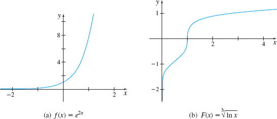
EXAMPLE 6Show that a Function Is Continuous
Show that:
- (a) f(x) = e^{2x} is continuous for all real numbers.
- (b) F(x) = \sqrt[3]{\ln x} is continuous for x>0.
Solution (a) The domain of the exponential function is the set of all real numbers, so f is defined for any number c. That is, f(c) = e^{2c}. Also for any number c, \begin{equation*} \lim\limits_{x\rightarrow c}f(x) = \lim\limits_{x\rightarrow c}e^{2x} = \lim\limits_{x\rightarrow c}(e^{x}) ^{2} = \left[ \lim\limits_{\kern.5ptx\rightarrow c}e^{x}\right] ^{2} = (e^{c}) ^{2} = e^{2c} = f(c) \end{equation*}
Since \lim\limits_{x\rightarrow c}f(x) = f(c) for any number c, then f is continuous at all numbers c.
(b) The logarithmic function f(x) = \ln x is continuous on its domain, the set of all positive real numbers. The function g(x) = \sqrt[3]{x} is continuous on its domain, the set of all real numbers. Then for any real number c>0, the composite function F(x) = (g\circ f) (x) = \sqrt[3]{\ln x} is continuous at c. That is, F is continuous at all numbers x>0.
Figures 45(a) and 45(b) illustrate the graphs of f and F.
NOW WORK
Summary
Basic Limits involving trigonometric, exponential, and logarithmic functions:
- \lim\limits_{x\rightarrow c}\sin x = \sin c
- \lim\limits_{x\rightarrow c}\cos x = \cos c
- \lim\limits_{\theta \rightarrow 0}\dfrac{\sin \theta}{\theta} = 1
- \lim\limits_{\theta \rightarrow 0}\dfrac{\cos \theta -1}{\theta} = 0
- \lim\limits_{x\rightarrow c}a^{x} = a^{c}
- \lim\limits_{x\rightarrow c}\log _{a}x = \log _{a}c, c>0