6.8 Center of Mass; Centroid; the Pappus TheoremPrinted Page 458
458
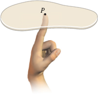
Anytime you have been able to balance an object on your fingertip, you have located its center of mass. See Figure 64. The center of mass of an object or a system of objects is the point that acts as if all the mass is concentrated at that point.
1 Find the Center of Mass of a Finite System of ObjectsPrinted Page 458
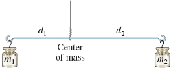
We begin with a system of two objects with masses m1 and m2 that are placed on the ends of a nearly weightless rod of length d that is hung from a wire. When the wire is placed at the center of mass of the objects, the rod will be horizontal. Mathematically, the rod is balanced, or in equilibrium, when m1d1=m2d2
where d1 and d2 are the distances of the objects from the vertical wire, as shown in Figure 65. The quantities m1d1 and m2d2, called moments, represent the tendency of the objects to rotate about the balancing point. When m1d1=m2d2, the tendency of the objects to rotate is equal, so no rotation occurs and equilibrium is attained.
If the rod were placed on a positive x-axis, as in Figure 66, with mass m1 at x1, mass m2 at x2, and the center of mass at ˉx, then the rod is balanced when m1(ˉx−x1)=m2(x2−ˉx)m1ˉx−m1x1=m2x2−m2ˉx(m1+m2)ˉx=m1x1+m2x2
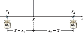
The center of mass ˉx of the two objects satisfies the equation ˉx=m1x1+m2x2m1+m2
EXAMPLE 1Finding the Center of Mass of a System of Objects on a Line
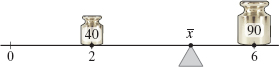
Find the center of mass of the system when a mass of 90 kg is placed at 6 and a mass of 40 kg is placed at 2.
Solution The system is shown in Figure 67, where the two masses are placed on a weightless seesaw. The center of mass ˉx will be at some number where a fulcrum balances the two masses. Then for equilibrium, ˉx=m1x1+m2x2m1+m2=40(2)+90(6)40+90=620130≈4.769
The center of mass is at ˉx≈4.769.


NOW WORK
459
The formula for the center of mass of two objects can be extended to any number n of objects.
Center of Mass of a System of n Objects on a Line
If n objects with masses m1,m2,…,mn are placed on a line at x1,x2,…,xn, respectively, then for equilibrium (m1+m2+⋯+mn)ˉx=m1x1+m2x2+⋯+mnxn
and the center of mass is ˉx, where ˉx=m1x1+m2x2+⋯+mnxnm1+m2+⋯+mn=n∑i=1(mixi)n∑i=1mi=n∑i=1(mixi)M
where M=n∑i=1mi is the mass of the system.
The numbers m1x1, m2x2,…,mnxn are called the moments about the origin of the masses m1, m2,…,mn. So, the center of mass ˉx is found by adding the moments about the origin and dividing by the total mass M of all the objects.
Now suppose the objects are not in a line, but are scattered in a plane.
Center of Mass of a System of n Objects in a Plane
If n objects m1,m2,…,mn are located at the points (x1,y1), (x2,y2),…,(xn,yn) in a plane, then the center of mass of the system is located at the point (ˉx,ˉy), where ˉx=n∑i=1(mixi)Mˉy=n∑i=1(miyi)M
and M=n∑i=1mi is the mass of the system.
The sum My=n∑i=1(mixi) is called the moment of the system about the y-axis and the sum Mx=n∑i=1(miyi) is called the moment of the system about the x-axis. The center of mass formulas then can be written as ˉx=MyMˉy=MxM
Physically, My measures the tendency of the system to rotate about the y-axis; Mx measures the tendency of the system to rotate about the x-axis.
EXAMPLE 2Finding the Center of Mass of a System of Objects in a Plane
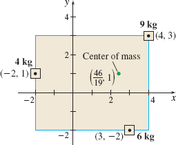
Find the center of mass of the system of objects having masses 4, 6, and 9 kg, located at the points (−2,1),(3,−2), and (4,3), respectively.
Solution See Figure 68. Where is a good estimate for the center of mass? Certainly, it will lie within the rectangle −2≤x≤4; −2≤y≤3.
460
To find the exact position of the center of mass, we first find the moment of the system about the y-axis, My, and the moment of the system about the x-axis, Mx. My=3∑i=1mixi=4(−2)+6(3)+9(4)=46Mx=3∑i=1miyi=4(1)+6(−2)+9(3)=19
Since the mass M of the system is M=4+6+9=19, we have ˉx=MyM=4619,ˉy=MxM=1919=1
The center of mass of these objects is at the point (4619,1). Notice that the center of mass lies in the rectangle −2≤x≤4; −2≤y≤3.
NOW WORK
2 Find the Centroid of a Homogeneous LaminaPrinted Page 460
With the formulas (1), we can approximate the center of mass of a thin, flat sheet of material, called a lamina, and express its center of mass in terms of definite integrals. We will assume that matter is continuously distributed throughout the lamina; that is, the mass density function ρ is continuous on the domain of the lamina. In the special case where the mass density function ρ is a constant function, the lamina is called homogeneous.
The mass of a homogeneous lamina is ρA, where A is the area of the lamina and ρ is its constant mass density. The center of mass of a homogeneous lamina is located at the centroid, the geometric center of the lamina.
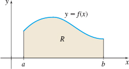
Suppose a homogeneous lamina is determined by a region R bounded by the graph of a function f, the x-axis, and the lines x=a and x=b. Also suppose that f is continuous and nonnegative on the closed interval [a,b]. See Figure 69.
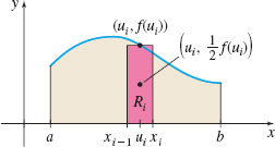
As before, we partition the interval [a,b] into n subintervals: [a,x1],[x1,x2],…,[xi−1,xi],…,[xn−1,b]a=x0b=xni=1,2,…,n each of width Δx=b−an, and select a number ui in each subinterval. Here, we choose ui to be the midpoint of the ith subinterval. That is, ui=xi−1+xi2
The lamina is now partitioned into n nonoverlapping rectangular regions, Ri, where i=1,2,…,n, each of which is a homogeneous lamina. From the symmetry of a rectangle, the centroid of Ri is (ui,12f(ui)). See Figure 70.
The mass mi of Ri is mi=ρAi=ρf(ui)Δx
The moment of Ri about the y-axis, My(Ri), is the product of the mass of Ri and the distance from (ui,12f(ui)) to the y-axis, which is ui. Then My(Ri)=miui=[ρf(ui)Δx]ui=ρuif(ui)Δx
Summing the n moments gives an approximation of the moment My of the lamina about the y-axis. That is, My≈ρn∑i=1uif(ui)Δx
461
As the number n of subintervals increases, the sums ρn∑i=1uif(ui)Δx become better approximations of My. These sums are Riemann sums, and since f is continuous on [a,b], the limit of the sums is a definite integral. That is, My=ρ∫baxf(x) dx
Similarly, the moment of Ri about the x-axis, Mx(Ri), is the product of its mass and the distance from the point (ui,12f(ui)) to the x-axis, which is 12f(ui). Mx(Ri)=mi[12f(ui)]=ρf(ui)Δx[12f(ui)]=12ρ[f(ui)]2Δx
Again, adding these moments gives an approximation of the moment Mx of the lamina about the x-axis, and as the number of subintervals increases, the sums 12ρn∑i=1[f(ui)]2Δx become better approximations of Mx. Since the sums are Riemann sums and f is continuous on [a,b], we have Mx=12ρ∫ba[f(x)]2 dx
For the region R, the mass of a homogeneous lamina is M=ρ∫baf(x) dx
Then the centroid (ˉx,ˉy) is given by ˉx=MyM=ρ∫baxf(x) dxρ∫baf(x) dx=∫baxf(x) dx∫baf(x) dx=∫baxf(x) dxA
and ˉy=MxM=12ρ∫ba[f(x)]2 dxρ∫baf(x) dx=12∫ba[f(x)]2 dx∫baf(x) dx=∫ba[f(x)]2 dx2A
where A=∫baf(x)dx is the area under the graph of f from a to b.
The Centroid of a Homogeneous Lamina
Let R be a lamina with a constant mass density ρ. If R is bounded by the graph of a function f, the x-axis, and the lines x=a and x=b, where f is continuous and nonnegative on the closed interval [a,b], then the centroid (ˉx,ˉy) of R is ˉx=1A∫baxf(x) dxˉy=12A∫ba[f(x)]2dx
where A=∫baf(x)dx
is the area under the graph of f from a to b.
462

EXAMPLE 3Finding the Centroid of a Homogeneous Lamina
Find the centroid of the homogeneous lamina bounded by the graph of f(x)=x2, the x-axis, and the line x=1.
Solution The lamina is shown in Figure 71.
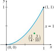
The area A of the lamina is A=∫10x2dx=[x33]10=13
Using formulas (2), the centroid of the lamina is ˉx=1A∫10xf(x) dx=113∫10 x⋅x2dx=3∫10x3dx=3[x44]10=34ˉy=12A∫10[f(x)]2dx=123∫10(x2)2dx=32∫10x4dx=32[x55]10=310
The centroid of the lamina is (34,310).
EXAMPLE 4Finding the Centroid of a Homogeneous Lamina
Find the centroid of one-quarter of a circular plate of radius R.
Solution We place the quarter-circle in the first quadrant, as shown in Figure 72(a). The equation of the quarter circle can be expressed as f(x)=√R2−x2, where 0≤x≤R.
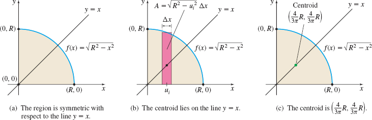
If you guessed that because the quarter of the circular plate is symmetric with respect to the line y=x, the centroid will lie on this line, you are correct. See Figure 72(b). So, ˉx=ˉy. The area A of the quarter circular region is A=πR24. ˉx=1A∫ba[xf(x)]dx=1A∫R0x√R2−x2dxˉy=12A∫ba[f(x)]2dx=12A∫R0(R2−x2)dx
463
Since ˉx=ˉy, and ˉy is easier to find, we evaluate ˉy. ˉx=ˉy=12A∫R0(R2−x2)dx=12(πR24)[R2x−x33]R0=2πR2(23R3)=43πR
The centroid of the lamina, as shown in Figure 72(c), is (ˉx,ˉy)=(43πR,43πR).
Example 4 illustrates the symmetry principle: If a homogeneous lamina is symmetric about a line L or a point P, then the centroid of the lamina lies on L or at the point P.
EXAMPLE 5Finding the Centroid of a Homogeneous Lamina
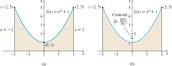
Find the centroid of the lamina bounded by the graph of y=f(x)=x2+1, the x-axis, and the lines x=−2 and x=2.
Solution Figure 73(a) shows the graph of the lamina.
We notice two properties of f.
- The graph of f is symmetric about the y-axis, so by the symmetry principle, ˉx=0.
- f is an even function, so ∫2−2f(x) dx=2∫20f(x) dx.
The area A of the region is A=2∫20(x2+1) dx=2[x33+x]20=2(83+2)=283 Using (2), we get ˉy=12A∫ba[f(x)]2dx=12A∫2−2[f(x)]2dx=12A⋅2∫20[f(x)]2dx=328∫20(x2+1)2dx=328∫20(x4+2x2+1) dx=328[x55+2x33+x]20=328(325+163+2)=10370≈1.471
The centroid of the lamina, as shown in Figure 73(b), is (ˉx,ˉy)=(0,10370).
Notice that the centroid in Example 5 does not lie within the lamina.
NOW WORK
464
In general, laminas are not homogeneous. The Challenge Problems at the end of the section investigate the center of mass of a lamina for which the density of the material varies with respect to x. The more general case, where the density of a lamina varies with both x and y, requires double integration and is treated in Chapter 14.
3 Find the Volume of a Solid of Revolution Using the Pappus TheoremPrinted Page 464
IN WORDS
The volume of a solid formed by revolving a plane region around an axis equals the product of area of the region and the distance its centroid travels around the axis.
THEOREM The Pappus Theorem for Volume
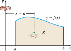
Let R be a plane region of area A and let V be the volume of the solid of revolution obtained by revolving R about a line that does not intersect R. Then the volume V of the solid of revolution is V=2πAd
where d is the distance from the centroid of R to the line.
Proof
We give a proof for the special case where the region R is bounded by the graph of a function f that is continuous and nonnegative on the interval [a,b], the x-axis, and the lines x=a and x=b, and where R is revolved about the y-axis, as shown in Figure 74. Using the shell method to find the volume of the solid of revolution and the centroid formula (2) for ˉx, we find V=↑Shell Method2π∫baxf(x)dx=↑(2)2π(Aˉx)=2πAd
where ˉx=d is the distance of the centroid (ˉx,ˉy) of R from the y-axis.
ORIGINS
The Greek mathematician Pappus of Alexandria (c. 300 AD) produced a mathematical collection containing a record of much of classical Greek mathematics. In it he shows a relationship between volume and centroids.
EXAMPLE 6Using the Pappus Theorem for Volume
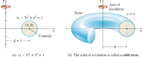
Use the Pappus Theorem to find the volume of the solid formed by revolving the region enclosed by the circle (x−3)2+y2=1 about the y-axis.
Solution By symmetry, the centroid of a circular region is the center of the circle. Here, the centroid is the point (3,0). See Figure 75(a).
NOTE
A torus is a doughnut-shaped surface.
The distance d from the centroid to the axis of revolution, which is the y-axis, is d=3. The area of the circle is A=πR2=π⋅12=π. It follows from the Pappus Theorem that the volume V of the solid of revolution [Figure 75(b)] is V=2π⋅(Area of the circle)⋅d=2π⋅π⋅3=6π2≈59.218 cubic units.
IN WORDS
A disk moving in a circle generates a solid torus. The volume of the torus equals the product of the circumference of the circle traveled by the centroid of the generating disk and the area of the disk.